Concepts

Communication services, layer models, protocols
Physical basics of transmission
Error handling and medium access
Internet Protocol (IP) and Routing: Connecting remote hosts
Transmission Control Protocol (TCP): Connecting applications
Security: Cryptographic primitives, IPsec, SSL/TLS

Client/Server- und Peer-to-Peer-Systeme
OSI-Referenzmodell und TCP/IP-Referenzmodell
Übertragungsmedien und Signaldarstellung
Fehlerbehandlung, Flusssteuerung und Medienzugriff
Lokale Netze, speziell Ethernet
Netzkomponenten und Firewalls
Internet-Protokolle: IP, Routing, TCP/UDP
Sicherheitsmanagement und Datenschutz, Sicherheitsprobleme und Angriffe im Internet
Grundlagen der Kryptographie und sichere Internet-Protokolle

What every CS major should know

Networking

Given the ubiquity of networks, computer scientists should have a firm understanding of the network stack and routing protocols within a network.

The mechanics of building an efficient, reliable transmission protocol (like TCP) on top of an unreliable transmission protocol (like IP) should not be magic to a computer scientist. It should be core knowledge.

Computer scientists must understand the trade-offs involved in protocol design–for example, when to choose TCP and when to choose UDP. (Programmers need to understand the larger social implications for congestion should they use UDP at large scales as well.)

Specific recommendations

Given the frequency with which the modern programmer encounters network programming, it’s helpful to know the protocols for existing standards, such as:

802.3 and 802.11;
IPv4 and IPv6; and
DNS, SMTP and HTTP.

Computer scientists should understand exponential back off in packet collision resolution and the additive-increase multiplicative-decrease mechanism involved in congestion control.

Every computer scientist should implement the following:

an HTTP client and daemon;
a DNS resolver and server; and
a command-line SMTP mailer.

No student should ever pass an intro neworking class without sniffing their instructor’s Google query off wireshark.

It’s probably going too far to require all students to implement a reliable transmission protocol from scratch atop IP, but I can say that it was a personally transformative experience for me as a student.

Security

The sad truth of security is that the majority of security vulnerabilities come from sloppy programming. The sadder truth is that many schools do a poor job of training programmers to secure their code.

Computer scientists must be aware of the means by which a program can be compromised.

They need to develop a sense of defensive programming–a mind for thinking about how their own code might be attacked.

Security is the kind of training that is best distributed throughout the entire curriculum: each discipline should warn students of its native vulnerabilities.

Specific recommendations

At a minimum, every computer scientist needs to understand:

social engineering;
buffer overflows;
integer overflow;
code injection vulnerabilities;
race conditions; and
privilege confusion.

A few readers have pointed out that computer scientists also need to be aware of basic IT security measures, such how to choose legitimately good passwords and how to properly configure a firewall with iptables.

Cryptography

Cryptography is what makes much of our digital lives possible.

Computer scientists should understand and be able to implement the following concepts, as well as the common pitfalls in doing so:

symmetric-key cryptosystems;
public-key cryptosystems;
secure hash functions;
challenge-response authentication;
digital signature algorithms; and
threshold cryptosystems.

Since it’s a common fault in implementations of cryptosystems, every computer scientist should know how to acquire a sufficiently random number for the task at hand.

At the very least, as nearly every data breach has shown, computer scientists need to know how to salt and hash passwords for storage.

Specific recommendations

Every computer scientist should have the pleasure of breaking ciphertext using pre-modern cryptosystems with hand-rolled statistical tools.

RSA is easy enough to implement that everyone should do it.

Every student should create their own digital certificate and set up https in apache. (It’s surprisingly arduous to do this.)

Student should also write a console web client that connects over SSL.

As strictly practical matters, computer scientists should know how to use GPG; how to use public-key authentication for ssh; and how to encrypt a directory or a hard disk.

Linux commands

Base64 decode:

echo -n 'UGFzc3dvcmQ6' | base64 -d

Base64 encode:

echo -n 'Password:' | base64

Hex to decimal number:

printf "%d\n" 0xFF

Basics

hostname   # show or set the system's host name
hostname -I   # Display all network addresses of the host.
domainname   # show or set the system's NIS/YP domain name
ypdomainname   # show or set the system's NIS/YP domain name
nisdomainname   # show or set the system's NIS/YP domain name
dnsdomainname   # show the system's DNS domain name

Tools

TODO

telnet   # used for interactive communication with another host using the TELNET protocol (like ssh, but not encrypted, thus not secure)
traceroute   # measuring roundtrip times (RTT)
ip
ifconfig
ipconfig   # in Microsoft Windows
systemd-resolve --flush-caches   # dns cache

configuration

MTU, MSS

ifconfig | grep mtu   # MTU size (https://linuxhint.com/how-to-change-mtu-size-in-linux/)
ip a | grep mtu
ifconfig wlo1 mtu 1000 up   # change MTU size of interface "wlo1" to 1000 bytes (https://linuxhint.com/how-to-change-mtu-size-in-linux/)

Wireshark:

there is an MSS= in the [SYN] packet “Info” column or [SYN, ACK] packet “Info” column

History of MSS: superuser

MSS = MTU - IPHeaderLen - TCPHeaderLen
IP headers are 20 bytes long
typical TCP headers are 32 bytes long now
- resulting in a typical 1448 byte TCP MSS on a standard 1500 byte MTU Ethernet network (like Ubuntu3060)

On Ubuntu3060 the TCP Wireshark Lab trace showed [TCP Segment Len: 2896] which was larger than the MTU on Ubuntu3060 which was 1500!

This is because tso/gso was turned on. See Segmentation Offload. When I turned it off, Wireshark showed [TCP Segment Len: 1448].

More precisely: from stackoverflow:

# the MSS shrinks when IP/TCP options are added
MSS = MTU - (20 + len(IP Options)) - (20 + len(TCP Options))

Segmentation Offload

sources:

ethtool -k wlo1   # display current settings for interface "wlo1"
sudo ethtool -K wlo1 gso off   # turn off gso
sudo ethtool -K wlo1 tso off   # turn off tso
sudo ethtool -K wlo1 tx-tcp-mangleid-segmentation on

ports, firewall

nmap   # port scanning

vim /etc/services   # port -> application map list

# There are two major firewalls in Ubuntu: ufw and firewalld
# always check both!
# phth: weil "iptables" Befehle zu kompliziert sind, hat man "ufw" und "firewalld" eingeführt

# Uncomplicated Firewall (ufw) 
# - frontend for "iptables" (https://wiki.ubuntu.com/UncomplicatedFirewall)
# - in Ubuntu 20.04 ufw is disabled by default 
#   - (why?: https://askubuntu.com/a/22739)
#     - in Ubuntu all ports are closed by default, thus no firewall is necessary
ufw   # opening/closing ports
sudo ufw allow 5201/tcp
sudo ufw delete allow 5201/tcp   # https://stackoverflow.com/a/37620498/12282296
sudo ufw enable   # always make sure ufw is enabled

# firewalld 
# - acts as an alternative to "nft" and "iptables" command line programs (https://en.wikipedia.org/wiki/Firewalld)
# - in Ubuntu 20.04 firewalld is not installed by default
systemctl status firewalld.service
service firewalld status   # same as "systemctl status firewalld.service"
service firewalld stop   # disable firewall (https://stackoverflow.com/a/51817241/12282296)
firewall-cmd --version   # check version
firewall-config   # gui for firewalld
firewall-applet   # tray applet for firewalld (installing this will also install firewall-config)

Measurements

traceroute   # measuring roundtrip times (RTT)

# disable firewalld first!
iperf3   # measuring throughput (https://www.cyberciti.biz/faq/how-to-test-the-network-speedthroughput-between-two-linux-servers/)

Throughput testing (iperf3)

TODO

First, disable any firewall. See ports, firewall.

On the server (receiver):

# iperf SERVER MODE
iperf3 -s

On the client (sender):

# iperf CLIENT MODE
# -c: The client mode can be started using the -c command-line option, which also
#     requires a host to which iperf3 should connect.  The host can be speci‐
#     fied by hostname, IPv4 literal, or IPv6 literal:
#
#            iperf3 -c iperf3.example.com
#
#            iperf3 -c 192.0.2.1
#
#            iperf3 -c 2001:db8::1
#
iperf3 -c server

# -p: If the iperf3 server is running on a non-default TCP  port,  that  port
#     number needs to be specified on the client as well:
#
iperf3 -c server -p port

Capture with Wireshark on the sending side!

tshark

phth: “Wireshark in command line.”

source:

TShark is a network protocol analyzer.
It lets you capture packet data from a live network, or read packets from a previously saved capture file, either printing a decoded form of those packets to the standard output or writing the packets to a file.
TShark is able to detect, read and write the same capture files that are supported by Wireshark.

Get the Field Name

right click on a field and select “Copy” → “Field Name” to get the field names for tshark syntax
- e.g. doing this on [The RTT to ACK the segment was: 0.000048281 seconds] will give you tcp.analysis.ack_rtt

Examples

tshark -r myfile.pcap -Y 'ip.addr == AA.BB.CC.DD' -T fields -e tcp.analysis.ack_rtt

from stackoverflow:
- to get the values of the RTT calculated by wireshark/tshark

Wireshark

Must-Knows

right click on a field and select “Apply as Column” to quickly see that fields value for all packets in the “Packet List” pane
View/Layout: “Edit” → “Preferences …” → “Appearance” → “Layout”

Wireshark GUI meaning

The “Packet List” Pane

the lines in the “No.” column connecting the selected packet with other packets (see Table 3.16. Related packet symbols)
- DNS packets that use the same port numbers. Wireshark treats them as belonging to the same conversation and draws a line connecting them.

TCP

RTT Graph

Statistics → TCP Stream Graph → Round Trip Time Graph
plots the RTT for each of the TCP segments sent
the plotted RTT values are in the field [SEQ/ACK analysis] → [The RTT to ACK the segment was: x.xxx seconds] (only visible in ACKs)
- see stackoverflow

Time-Sequence-Graph (Stevens)

plots sequence numbers with respect to time
if there are no retransmitted segments, the sequence numbers from the source to the destination should be increasing monotonically with respect to time

Time-Sequence-Graph (tcptrace)

watch
- helps to see congestion and rwnd
- helps to see lost packets, retransmissions, SACKs

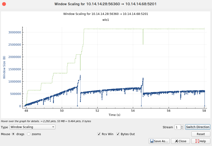
“Window Scaling” Graph

“Statistics” → “TCP Stream Graphs” → “Window Scaling” shows rwnd (green line) and “[Bytes in flight:]” (blue points) (see Figure 9)
watch: “Bytes in flight”

Measure Throughput

total data: difference between the sequence number of the first TCP segment and the acknowledged sequence number of the last ACK
total transmission time: difference of the time instant of the first TCP segment and the time instant of the last ACK
throughput = total data / total transmission time

Fields

[SEQ/ACK analysis]:
- for ACKs: contains e.g.
  - [This is an ACK to the segment in frame: 98] (must: right click → “Apply as Column”)
  - [The RTT to ACK the segment was: 0.000048281 seconds]
- for SEQs: contains e.g.
  - [Bytes in flight: 5120], i.e. “outstanding data” (for Wireshark Lab TCP “estimate cwnd” task: “Apply as Column”)
    - can be used to estimate a lower bound for the cwnd size (see Wireshark Lab TCP)
      - watch: “TCP congestion control”
    - Ubuntu3060: builds up in MSS units after the handshake, i.e. it starts with 2 MSS (2896 bytes), 4 MSS (5792 bytes), 6 MSS (8688 bytes), etc.
      - after some bytes have been ACKed this number is not a multiple of the MSS size any more!
    - the “Window Scaling” Graph visualizes this field
      - watch: “Bytes in flight”
- for “Bad TCP” packets (black colored packets, red font): contains e.g.
  - [TCP Analysis Flags]
    - in [TCP Window Full] packets:
      - [Expert Info (Warning/Sequence): TCP window specified by the receiver is now completely full]
    - in [TCP ZeroWindow] packets:
      - [Expert Info (Warning/Sequence): TCP Zero Window segment]
      - Note: [TCP ZeroWindow] packets are followed by [TCP window update] packets, i.e. the receiver saying to the sender “I freed my receive window. You can start sending to me again.”. Only then the sender is allowed to proceed.
[Calculated window size: xyz]: the rwnd size (advertized by the receiver to the sender)
- nowadays, much more data is transferred, so that the Window size value is scaled by [Window size scaling factor: xyz], i.e. rwnd = [Calculated window size: 64256] = [Window size scaling factor: xyz] * Window size value

Figure 9: “Window Scaling” Graph, shows a simple throughput test via iperf3 (see throughput testing (iperf3))

OSI Model

Layer 1: Physical layer
Layer 2: Data link layer
Layer 3: Network layer
Layer 4: Transport layer
Layer 5: Session layer
Layer 6: Presentation layer
Layer 7: Application layer

Multiplexing

Circuit Switching (TDM or FDM)

In circuit switching network resources (bandwidth) are divided into pieces (using either TD multiplexing (TDM) or FD multiplexing (FDM))
bit delay is constant during a connection

Packet Switching (statistical multiplexing)

transfers the data to a network in form of packets (using statistical multiplexing)
unlike circuit switching, packet switching requires no pre-setup (saving time) or reservation of resources (saving resources)
from geeksforgeeks
- Packet Switching uses Store and Forward technique while switching the packets; while forwarding the packet each hop first stores that packet then forward.
  - This technique is very beneficial because packets may get discarded at any hop due to some reason.
  - More than one path is possible between a pair of sources and destinations. Each packet contains Source and destination address using which they independently travel through the network.
    - In other words, packets belonging to the same file may or may not travel through the same path. If there is congestion at some path, packets are allowed to choose different paths possible over an existing network.

The Internet

An Internet service provider (ISP) is an organization that provides services for accessing, using, or participating in the Internet.
Internet exchange points (IXes or IXPs) are common grounds of IP networking, allowing participant Internet service providers (ISPs) to exchange data destined for their respective networks

Tiers of networks

There is no authority that defines tiers of networks participating in the Internet
A Tier 1 network is a network that can reach every other network on the Internet without purchasing IP transit or paying for peering
A Tier 2 network is an Internet service provider which engages in the practice of peering with other networks, but which also purchases IP transit to reach some portion of the Internet.
- the most common Internet service providers, as it is much easier to purchase transit from a Tier 1 network than to peer with them and attempt to become a Tier 1 carrier
The term Tier 3 network is sometimes also used to describe networks who solely purchase IP transit from other networks to reach the Internet

Delay and Loss

packet delay
- transmission delay
  - takes some time to put the bits on the wire (or whatever the medium is)
- queueing delay
  - if there is a line, i.e. some packets are waiting to be sent, there will be a delay
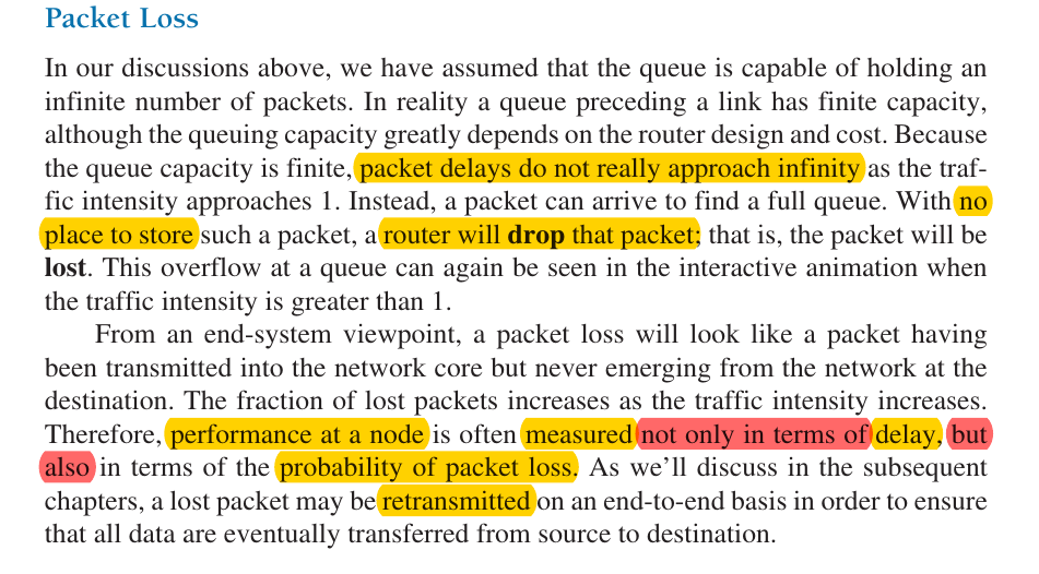
packet loss
- arriving packets will be dropped by the router, if the queue is full, i.e. if there are no free buffers (= storage)

Queueing Delay

can vary from packet to packet
- e.g., if 10 packets arrive at an empty queue at the same time, the first packet transmitted will suffer no queuing delay, while the last packet transmitted will suffer a relatively large queuing delay (while it waits for the other nine packets to be transmitted)
- therefore, one typically uses statistical measures, e.g.
  - average queuing delay
  - variance of queuing delay
  - probability that the queuing delay exceeds some specified value
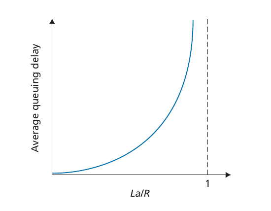
  - Notice, that Figure 8 plots the average delay! The actual delay will vary from packet to packet.
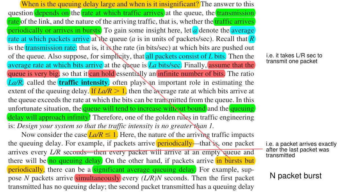
When is the queuing delay large and when is it insignificant?
- depends on
  - the rate at which traffic arrives at the queue,
  - the transmission rate of the link,
  - the nature of the arriving traffic,
    - that is, whether the traffic arrives periodically or arrives in bursts.
measuring queueing delay (see Figure 8):
- traffic intensity $=\frac{La}{R}$
  - $R=$link bandwidth
  - $L=$packet length
  - $a=$average packet arrival rate
- see graph in Figure 7 bottom right:
  - $= 0$: no delay
  - $\gt 1$: queue increases without bound $\Rightarrow$ infinite delay
  - $\leq 1$: depends on the nature of the arriving traffic
    - periodic: $1$ packet every $\frac{L}{R}$ seconds: no delay
    - periodic bursts: $N$ packets every $N \frac{L}{R}$ seconds: no delay for 1st packet, large delay for $N$th packet
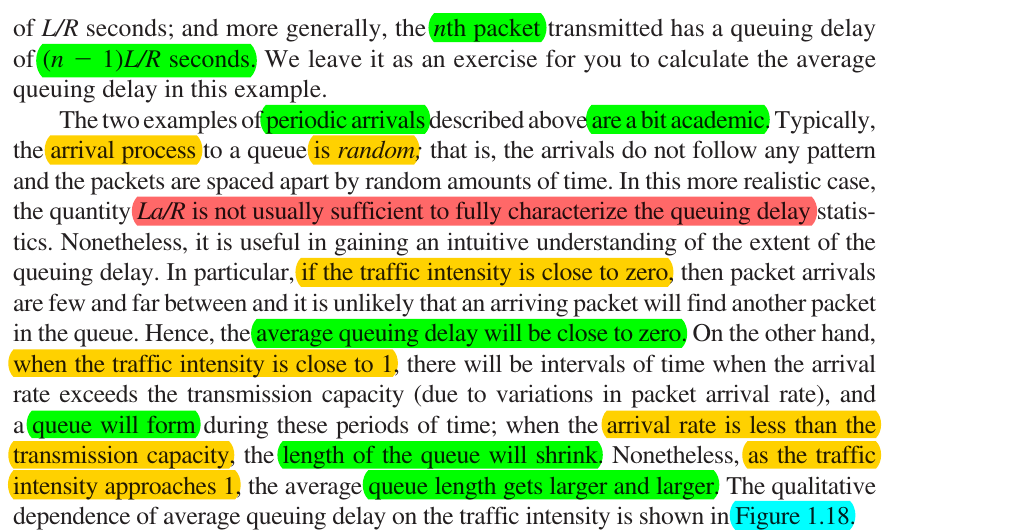
    - real world: random arrival
for $\gt 1$ the delay does not really approach infinity, instead the router drops packets (packet loss) because there is no storage available

Figure 8: average queueing delay

Application layer (Brief)

ip address: identifies a specific host
port: identifies a specific process
- e.g. http servers/web servers run on port 80
  - when browsers want http files, they will send a message to the ip address of the server and the port number associated with http, i.e. port 80

Transport layer (Brief)

Transport protocols: TCP/UDP

TCP
- connection-oriented: sets up a connection between client and server processes (thus, there is some overhead to set this up initially)
- reliable: makes sure there is no packet loss (requires some extra information to be sent, i.e. reliability requires some extra bandwidth)
- flow control: slows down the sender because the receiver is overloaded
- congestion control: slows down the sender because the network (in between the sender and receiver) is overloaded
UDP
- connection-less: no setting up, thus no overhead
- unreliable: no guarantees that a sent packet will arrive or will be uncorrupted or will be unduplicated
- no flow control
- no congestion control
note: UDP is faster and gives you more control over the trade-offs you want to make than TCP. If you need reliability, flow control or congestion control you could implement it yourself at the application layer. For some apps UDP makes more sense, e.g. internet telephony, streaming video.
- from wiki: “Voice and video traffic is generally transmitted using UDP”

Application Layer (Layer 7)

Web and HTTP

TODO

WebSocket

WebSocket Wikipedia:

a computer communications protocol, providing full-duplex communication channels over a single TCP connection.
the corresponding API: “WebSockets”
- a living standard maintained by the WHATWG and
- a successor to “The WebSocket API” from the W3C

WebSocket vs HTTP, Wikipedia:

WebSocket is distinct from HTTP.
Both protocols are located at layer 7 in the OSI model and depend on TCP at layer 4.
Although they are different, RFC 6455 states that WebSocket “is designed
- to work over HTTP ports 443 and 80 as well as
- to support HTTP proxies and intermediaries”, thus making it compatible with HTTP.
To achieve compatibility, the WebSocket handshake uses the HTTP Upgrade header to change from the HTTP protocol to the WebSocket protocol.
The WebSocket protocol enables interaction between a web browser (or other client application) and a web server with lower overhead than half-duplex alternatives such as HTTP polling, facilitating real-time data transfer from and to the server.

Email

SMTP

Using app passwords in Gmail: “When you use 2-Step Verification, some less secure apps or devices may be blocked from accessing your Google Account. App Passwords are a way to let the blocked app or device access your Google Account.”

Mostly from stackoverflow:

# must use -ign_eof flag here, otherwise the "R" in RCPT TO line will cause "RENEGOTIATING"
# (see https://stackoverflow.com/questions/59956241/connection-with-google-mail-using-openssl-s-client-command)
$ openssl s_client -connect smtp.gmail.com:465 -ign_eof

HELO smtp

auth login

# get username in base64 encoding 
# (sidenote: in order to *DE*code simply use "base64 -d" instead of "base64" at the end of this command)
echo -n 'phrth2@gmail.com' | base64

# generate app password (see https://support.google.com/accounts/answer/185833?hl=en)
echo -n 'app_password' | base64

EHLO smtp
MAIL FROM: <phrth@gmx.de>
RCPT TO: <phrth2@gmail.com>
DATA

=== enter e-mail content ===

ctrl-v-enter enter
. ctrl-v-enter

DNS

A Distributed, Hierarchical Database
hierarchy:
- root DNS server (returns IP address of TLD server, e.g. for TLD .com)
- TLD server (returns IP address of authoritative server, e.g. authoritative for amazon.com)
  - Note: The TLD server does not always know the authoritative DNS server for the hostname! It may know only of an intermediate DNS server, which in turn knows the authoritative DNS server for the hostname.
    - e.g. an intermediate university DNS server and authoritative departmental DNS servers
- (intermediate DNS server)
- authoritative DNS server (returns the IP address for the hostname, e.g. for the hostname www.amazon.com)
  - most universities and large companies implement and maintain their own authoritative server
local DNS server (aka default name server):
- does not belong to the hierarchy
- each ISP has a local DNS server
- when a host connects to an ISP, the ISP provides the host with the IP addresses of one or more of its local DNS servers (via DHCP)
- typically close to the host (i.e. not more than a few routers away from the host)

Recursive vs Iterative DNS query

recursive DNS query: obtain the mapping on the querying DNS server’s behalf
iterative DNS query: replies are directly returned to the querying DNS server
in theory, any DNS query can be iterative or recursive
in practice, DNS queries typically follow the pattern in Fig. 2.19
- i.e. the query from the requesting host to the local DNS server is recursive, and the remaining queries are iterative

DNS Cache

In a query chain, when a DNS server receives a DNS reply (containing, for example, a mapping from a hostname to an IP address), it can cache the mapping in its local memory.
Timeout: Because hosts and mappings between hostnames and IP addresses are by no means permanent, DNS servers discard cached information after a period of time (often set to two days)
A local DNS server can also cache the TLD servers’ IP addresses
- In fact, because of caching, root servers are bypassed for all but a very small fraction of DNS queries

DNS Cache in Ubuntu, Time to Live (TTL)

From linuxhint.com and techrepublic.com:

Ubuntu caches DNS queries by default using systemd-resolved.

systemd-resolved is a systemd service that provides network name resolution to local applications via a local DNS stub listener on 127.0.0.53. (from wiki.archlinux)
- It implements a caching and validating DNS/DNSSEC stub resolver (from freedesktop.org)
Prior to systemd, there was almost no OS-level DNS caching, see stackexchange
- old Ubuntu versions used dnsmasq (A lightweight DHCP and caching DNS server) and nscd (name service cache daemon) instead of systemd-resolved

# check how many DNS entries are cached
sudo systemd-resolve --statistics

# flush the DNS cache
sudo systemd-resolve --flush-caches

# alternatively, restart the systemd-resolved service to flush the DNS caches
sudo systemctl restart systemd-resolved

# view the DNS cache contents
sudo killall -USR1 systemd-resolved
sudo journalctl -u systemd-resolved > ~/dns-cache.txt

First check, if DNS caching is enabled:

If DNS caching is enabled the DNS server used to resolve the domain name (e.g. when using nslookup domain_name) is a loopback IP address, e.g. 127.0.0.53. If you have it disabled, then the DNS server should be anything other than 127.0.0.X. - Why?: This is because the loopback ip address 127.0.0.X indicates that the service systemd-resolved (which caches DNS records) is running.

Then, in order to get TTL values:

nslookup -debug www.cyberciti.biz
nslookup -debug -type=NS google.com

dig +ttlunits A www.cyberciti.biz
dig +ttlunits NS google.com

# show the TTL only
dig +nocmd +noall +answer +ttlid A www.cyberciti.biz

DNS Resource Records (RRs)

a four-touple (Name, Value, Type, TTL), where Name and Value depend on the Type
If a DNS server is authoritative for a particular hostname, then the DNS server will contain a Type A record for the hostname.
- (Even if the DNS server is not authoritative, it may contain a Type A record in its cache.)
If a server is not authoritative for a hostname, then the server will contain a Type NS record for the domain that includes the hostname
- it will also contain a Type A record that provides the IP address of the DNS server in the Value field of the NS record.

nslookup, dig

Caution: dig and nslookup sometimes display different information. dig uses the OS resolver libraries. nslookup uses its own internal ones. ISC recommends to stop using nslookup (see stackexchange)!

nslookup: General syntax: nslookup –option1 –option2 host-to-find dns-server Options:

nslookup -debug: show additional information, e.g. TTL

dig: General syntax: dig [options] TYPE domain auth-name-server-here Options:

dig +short: short form answer
dig +ttlunits: human-readable time units
dig +nocmd +noall +answer +ttlid: show the TTL only

Example 1: Send me the IP address for the host www.mit.edu:

nslookup -type=A www.mit.edu
dig A www.mit.edu

Example 2: Send me the host names of the authoritative DNS servers for the domain mit.edu:

# note: mit.edu is a domain, so no "www."!
nslookup -type=NS mit.edu
dig NS mit.edu

Example 3: Query sent to the DNS server dns2.p08.nsone.net rather than to the default DNS server:

possible errors, when using nslookup:
- ** server can't find some_site.com: NXDOMAIN: the host-to-find is wrong
- ** server can't find some_site.com: REFUSED: the dns-server is wrong, more precisely:
  - nslookup from another name server
  - “Refused” doesn’t mean that the connection to the DNS server is refused. It means that the DNS server refuses to provide whatever data you asked for, or to do whatever action you asked it to do

nslookup www.google.com dns2.p08.nsone.net

# note: do not forget the @ symbol here!
dig www.google.com @dns2.p08.nsone.net

ip, ifconfig, ipconfig, nmcli, iwconfig

ipconfig is a Windows command, it displays slightly different information than ifconfig and ip
ifconfig is deprecated, use ip
sudo ifconfig wlo1 10.14.14.29 netmask 255.255.255.0 set an ip address (if you leave out the netmask 255.255.255.0, then the netmask will change!)
ip a, ip address, ip address show
ip r default gateway/router address
nmcli dev show wlo1 show gateway and DNS servers for device wlo1
nmcli dev status get device names and their status types
systemd-resolve --status | grep Current: currently used DNS server IP address (source)
sudo iwconfig wlan1 essid "myWifi" key "s:password" (without quotation marks) associate the wifi device with the Access Point

Loopback address, Localhost

From techopedia.com:

A loopback address has been built into the IP domain system in order to allow for a device to send and receive its own data packets.

Loopback addresses can be useful in various kinds of analysis like testing and debugging, or in allowing routers to communicate in specific ways.

A simple way of describing how using a loopback address works is that a data packet will get sent through a network and routed back to the same device where it originated.

In IPv4, 127.0.0.1 is the most commonly used loopback address, however, this can range be extended to 127.255.255.255.

From tutorialspoint.com:

The IP address range 127.0.0.0 – 127.255.255.255 is reserved for loopback, i.e. a Host’s self-address, also known as localhost address. This loopback IP address is managed entirely by and within the operating system. Loopback addresses, enable the Server and Client processes on a single system to communicate with each other. When a process creates a packet with destination address as loopback address, the operating system loops it back to itself without having any interference of NIC (wiki “NIC”: network interface controller (NIC, also known as a network interface card, network adapter, LAN adapter or physical network interface).

Data sent on loopback is forwarded by the operating system to a virtual network interface within operating system. This address is mostly used for testing purposes like client-server architecture on a single machine. Other than that, if a host machine can successfully ping 127.0.0.1 or any IP from loopback range, implies that the TCP/IP software stack on the machine is successfully loaded and working.

Why is such a large IPv4 range assigned to localhost? (from stackexchange)

At the time (1986), the internet was completely classful and nobody really gave much thought to allocating this much space to the loopback address. Thus, the loopback got an entire Class A network.

P2P File Distribution

Peer-to-peer (P2P) computing or networking is a distributed application architecture that partitions tasks or workloads between peers.

Peers are equally privileged, equipotent participants in the network.
They are said to form a peer-to-peer network of nodes.
Peers make a portion of their resources, such as processing power, disk storage or network bandwidth, directly available to other network participants, without the need for central coordination by servers or stable hosts.
Peers are both suppliers and consumers of resources, in contrast to the traditional client–server model in which the consumption and supply of resources are divided.

RTSP, WebRTC

Real Time Streaming Protocol
P2P video chat
- ready-to-use WebRTC/RTSP server ( rtsp-simple-server )

Transport Layer (Layer 4)

The Transport Layer (Layer 4) is about providing logical communication between processes. - logical: it will appear as if host A is talking to host B, even though in actuality they are going over lots of other hosts, intermediate links, routers etc. - in other words TCP and UDP are end to end protocols (and not “point to point”!)

The transport layer of the sender disassembles (multiplexes) the messages passed from the application layer into chunks and the receiver reassembles (demultiplexes) those messages.

The Network Layer (Layer 3) is about providing logical communication between hosts. - hosts: a generic name for computers or routers - point to point: where the points are the hosts

From quora:

End to end indicates a communication happening between two applications (maybe you and your friend using Skype). It doesn’t care what’s in the middle, it just consider that the two ends are taking with one another. It generally is a Layer 4 (or higher) communication
Point to point is a Layer 2 link with two devices only on it. That is, two devices with an IP address have a cable going straight from a device into the other. A protocol used there is PPP, and HDLC is a legacy one.
Hop by Hop indicates the flow the communication follows. Data pass through multiple devices with an IP address, and each is genetically named “hop”. Hop by Hop indicates analyzing the data flow at layer 3, checking all devices in the path

Analogy: - 2 houses - hosts - NY and LA - 12 siblings/house - processes - 1 letter/child/week - messages - Ann (NY) and Bill (LA) - transport layer - collect and distribute - Post office (PO) - network layer - delivers from NY PO to LA PO

The transport layer just connects processes to the network layer. The transport layer abstracts away all the complexity of the network layer (in the analogy: delivering may involve trucks, plane, etc. which is dealt with at the PO level, but Ann and Bill do not know these details).

TCP and UDP

neither of these provide delay guarantees or bandwidth guarantees

TCP

Reliable, In-Order
provides:
- congestion control (TCP slows itself down if network is congested)
- flow control (TCP sender will slow itself down if TCP receiver cannot keep up with the speed that it is sending)
- connection setup (requires time and resources to be set up ahead of time to create this TCP connection)
ensures that packets/segments are received reliably (i.e. they do not get lost) and they are received in order

UDP

Unreliable, Unordered
“Best Effort”, “no-frills”, “bare bones”
UDP is very much a “no-frills” extension of the internet protocol IP that it is sitting on top of
very little overhead
- no handshaking
- no connection establishment
  - no delay
- no connection state at sender, receiver
  - thus, small segment header, less wasted bandwidth
- no congestion control
  - thus, no speed limit
use cases:
- streaming multimedia
- DNS
- SNMP
  - Simple Network Management Protocol
  - protocol for collecting and organizing information about managed devices on IP networks and for modifying that information to change device behaviour
  - supported by: cable modems, routers, switches, servers, workstations, printers, and more
  - is a part of TCP/IP Suite
  - includes an application layer protocol, a database schema, and a set of data objects
if you need reliability you can add it at the application layer and do application specific error recovery

Multiplexing/Demultiplexing

socket: like a “door”, a connection piece that …
- sits in between the application and transport layer
- is the means by which processes communicate
- a process (as part of a network application) can have one or more sockets, doors through which data passes
  - from the network to the process and
  - from the process to the network
- the transport layer in the receiving host does not actually deliver data directly to a process, but instead to an intermediary socket
- each socket has a unique identifier
port number: distinguishing identifier - one of them - that we use to distinguish what process needs to get a message/segment
- 16-bit number (0 to 65535)
- well-known ports 0 to 1023 (RFC 3232 which replaced RFC 1700)
  - http: 80
  - https: 443
  - ssh: 22
  - ftp: 21
  - smtp: 25
  - dns: 53
  - Official List: Internet Assigned Numbers Authority (iana.org)

Segments, Datagrams, Messages (Encapsulation)

application layer message (application layer data unit)
transport layer segment format (transport layer data unit):
- width: 32 bits
- source port #, dest port #
- other header fields
- application data (message)
UDP segment format:
- source port # (16 bits), dest port # (16 bits)
- length (in bytes, incl. header and payload), checksum
- application data (message)
- UDP adds four fields (2 bytes each, i.e. 8 bytes in total) to the application data (message)
IP datagram format (network layer data unit):
- source IP address
- destination IP address
- TCP/UDP segment (see above)
difference between datagrams and segments (from quora):
- We say TCP segment is the protocol data unit which consists of a TCP header and an application data piece (packet) which comes from the (upper) Application Layer. Transport layer data is generally named as segment and network layer data unit is named as datagram, but when we use UDP as transport layer protocol we don’t say UDP segment, instead, we say UDP datagram. I think this is because we do not segmentate UDP data unit (segmentation is made in transport layer when we use TCP).
encapsulation:
- a datagram encapsulates a segment which encapsulates a message
from TCP Wireshark Lab:
- why TCP Segment Len: 1460 ?
  - typically, the interface card limits the length of the maximum IP datagram to 1500 bytes, and there is a minimum of 40 bytes of TCP/IP header data
see MSS

Payload

From Kurose, Ross:

At each layer, a packet has two types of fields:

header fields
a payload field
- typically a packet from the layer above

Demultiplexing

Connectionless Demultiplexing (UDP):
- UDP socket identified by 2-tuple
  - the destination port (DP) and
  - the destination IP address
- the source port (SP) and the source IP address are not relevant for UDP demultiplexing, but they provide the return address (i.e. SP and DP will be swapped around, when talking back)
  - thus, a server can demultiplex messages from two hosts, even if those happen to have the same SP (cf. Fig. 3.5 Kurose)
Connection-Oriented Demultiplexing (TCP):
- TCP socket identified by 4-tuple
  - the SP and
  - the source IP address
  - the DP and
  - the destination IP address

Checksum

ones’ complement of the sum of all the 16-bit words in the UDP segment
- why we use 1’s complement instead of 2’s complement
  - because using 2’s complement may give you a wrong result if the sender and receiver machines have different endianness
checksum of sender and receiver is compared by addition (their sum must be zero!)
at the link layer cyclic redundancy check (CRC) is used
- because algorithm above fails to detect some common errors which affect many bits at once, such as
  - changing the order of data words, or
  - inserting or deleting words with all bits set to zero
Why is the link layer checksum not enough?
- no guarantees that the link layer is reliable and does the checksum
- End-to-End principle

Ones’ Complement

terminology: bit flip = bitwise NOT = ones’ complement of a binary number

Two’s Complement

“1 added to the ones’ complement”
Two’s complement
- (in maths) operation to reversibly convert a positive binary number into a negative binary number with equivalent (but negative) value, using the binary digit with the greatest place value to indicate whether the binary number is positive or negative (the sign)
- is executed by 1) inverting (i.e. flipping) all bits, then 2) adding a place value of 1 to the inverted number
- most common method of representing signed integers
  - in two’s complement, there is only one representation for zero, whereas in ones’ complement there are two (this is the reason why two’s complement is generally used) source

Endianness

A big-endian system stores the most significant byte (MSB) of a word at the smallest memory address.

End-to-End Principle

see

Basic design principle of the internet: “keep the core simple”.

There are many different phrasings:

“Communication protocol operations should be defined to occur at the endpoints of a communication system.”
Saltzer 1984: “The principle, called the end-to-end argument, suggests that functions placed at low levels of a system may be redundant or of little value when compared with the cost of providing them at that low level.”

Examples of this principle:

TCP checksum vs. application checksum
“smart” TCP vs “dumb” IP
- IP is “below” TCP
- IP is “dumb” in the sense that it has not many features compared to TCP

Principles of Reliable Data Transfer

FSM notation: (see rdt1.0 introduction)
- Lambda: “no action” or “no event”
- dashed arrow: initial state of the FSM
rdt1.0: reliable transfer over a reliable channel: no bit errors, no packet loss
- FSM:
  - sender:
    - 1 state: “wait for call from above”
  - receiver:
    - 1 state: “wait for call from below”
rdt2.0: channel with bit errors (stop-and-wait protocol)
- checksum to detect bit errors
- ACKs and NAKs (without errors!)
- retransmit on receipt of NAK
- FSM changes wrt rdt1.0:
  - sender:
    - 2 states: “wait for call from above” and “wait for ACK or NAK”
  - receiver:
    - 1 state: “wait for call from below”
rdt2.1: corrupted ACKs/NAKs (watch: Kurose)
- sender
  - if ACK/NAK corrupted: retransmit current packet
  - add sequence number to each packet
- receiver
  - discard (= do not deliver up) duplicate packets
- FSM changes wrt rdt2.0:
  - sender:
    - 4 states (because 2 sequence numbers)
  - receiver:
    - 2 states (because 2 sequence numbers)
rdt2.2: a NAK-free protocol (similar to TCP) (watch: Epic Networks Lab)
- same as rdt2.1, using ACKs only
- the sequence number of the packet being ACKed is in the ACK’s header
- receiver
  - keeps resending the ACK for the last packet that it received correctly
- sender
  - sees duplicate ACKs,
  - goes back and
  - resends the next packet after the one received correctly
- FSM changes wrt rdt2.1:
  - same number of states as rdt2.1
  - sender:
    - instead of “ACK or NAK”: check if ACK for 0 or ACK for 1
    - if ACK, but not for the packet that is expected: resend last packet
  - receiver:
    - if “waiting for 0” and it gets
      - a corrupt packet or seq1: send ACK for 1 (i.e. last packet that it received correctly)
      - the expected packet: send ACK for 0 (i.e. the expected packet)
rdt3.0: channel with errors and loss (stop-and-wait protocol)
- FSM changes wrt rdt2.2:
  - same number of states as rdt2.2
  - sender:
    - while in the “waiting for” state
      - timeout: resend
      - if corrupt packet or wrong sequence number do not do anything, just wait for timeout
- performance problem with rdt3.0: Utilization
  - solution: Pipelining

Sequence Numbers

in rdt2.1 and all following rdts
watch original lecture video to understand sequence numbers
- they explain them differently than Kenan Casey
- both the sender and the receiver expect a certain sequence number (0 or 1) which does not have to be the same for the sender and the receiver

Utilization

watch: Epic Networks Lab
$D_{prop}_{}$: propagation delay (one way, i.e. sender to receiver, but not back!)
- $D_{prop}_{} = 15\;\text{ms}$
$\text{RTT}$: Roundtrip time (both ways)
- $\text{RTT} = 2 \times 15\;\text{ms}$
$D_{trans}_{}$: transmission delay
- $D_{trans}_{} = \frac{L}{R} = \frac{8000\;\text{bits}}{1\;\text{Gbps}} = 8\;\mu s$
  - Note: $8000\;\text{bits} = 1000\;\text{bytes}$
the transmission delay is much smaller relative to the propagation delay
$U$: fraction of time sender busy sending
- ideal protocol: $U = 1$
- $U = \frac{\frac{L}{R}}{\text{RTT} + \frac{L}{R}} = \frac{.008}{30.008} = 0.00027$
  - Thus, rdt3.0 has very low utilization! This is why pipelining is necessary!

Pipelining

watch: Epic Networks Lab
sender allows multiple, “in-flight”, yet-to-be-acknowledged packets
- range of sequence numbers must be increased
  - the range will depend on the approach (i.e. GBN or Selective Repeat)
- buffering (= saving) of more than one packet at sender and/or receiver
  - buffer = save (see KR 3.4.3 “GBN” p. 219)
more utilization by “filling the pipe”
- $U_{sender}_{} = \frac{3\frac{L}{R}}{\text{RTT} + \frac{L}{R}} = \frac{.024}{30.008} = 0.00081$
2 common ways of pipelined error recovery
- Go-Back-N
- Selective Repeat
both algorithms were optimized to need as few pointers and timers as possible (resources were far more scarce back then)

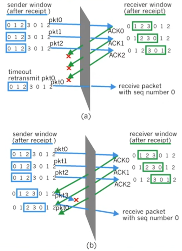
Go-Back-N (sliding-window protocol)

just play with Kurose animations:
- GBN
- e.g. send 3 packets, kill packet 1 and wait for the timeout and see what happens

Sender

window of up to N consecutively transmitted but unACKed packets
2 state variables:
- base: sequence number of the oldest unacknowledged packet
- nextseqnum: smallest unused sequence number (sequence number of the next packet to be sent)
cumulative ACK: ACK for a packet with sequence number $n$ will be taken to be a cumulative ACK
- i.e. the sender assumes that this ACK with sequence number $n$ indicates that all packets with a sequence number up to and including $n$ have been correctly received at the receiver
timer for oldest in-flight packet
- timeout: resend all packets that have been previously sent but that have not yet been acknowledged
- restart timer: ACK received but there are still outstanding packets
- stop timer: ACK received and no outstanding packets
Why limit N?
- see TCP discussion below
- flow control
- congestion control
sequence number is carried in a fixed-length field in the packet header
- If $k$ is the number of bits in the packet sequence number field, the range of sequence numbers is thus $i\left[ 0, 2k - 1 \right]$
- With a finite range of sequence numbers, all arithmetic involving sequence numbers must then be done using modulo $2k$ arithmetic
  - i.e. the sequence number space can be thought of as a ring of size $2k$, where sequence number $2k - 1$ is immediately followed by sequence number $0$
- rdt3.0: 1-bit sequence number
- TCP: 32-bit sequence number
  - TCP sequence numbers count bytes in the byte stream rather than packets
    - sequence number as a “byte counter”

Receiver

1 state variable:
- expectedseqnum: sequence number of the next in-order packet
If a packet with sequence number $n$ is received correctly and is in order (i.e. data last delivered to upper layer came from a packet with seq $n - 1$),
- the receiver sends an ACK for packet $n$ and delivers the data portion of the packet to the upper layer.
In all other cases,
- the receiver discards the packet and resends an ACK for the most recently received in-order packet.
discarding out-of-order packets
- advantage:
  - simplicity of receiver buffering
    - the only piece of information the receiver need maintain is the sequence number of the next in-order packet expectedseqnum
- disadvantage:
  - the subsequent retransmission of that packet might be lost or garbled and thus even more retransmissions would be required
(Note: In some implementations the receiver may buffer out-of-order packets instead of discarding them.)
experiments with GBN animation:
- experiment 1 (see images below):
  - send 3 packets (press three times “Send New”)
  - press “Pause”
  - select the packet in the middle (packet number 1, see numbers on top of the packets) and “Kill Packet”
  - press “Resume”
- observation 1 (see Figure 2):
  - in addition to the ACK for the in-order packet 0, the receiver sends a second ACK for the packet last sent (packet number 2), too
    - reason: Look closely at the numbers on top of the ACKs. Both ACKs have sequence number 0, the number of the most recently received in-order packet! Thus, the first ACK with sequence number 0 has been resent!

Figure 1: packet 1 is lost pre_ACK

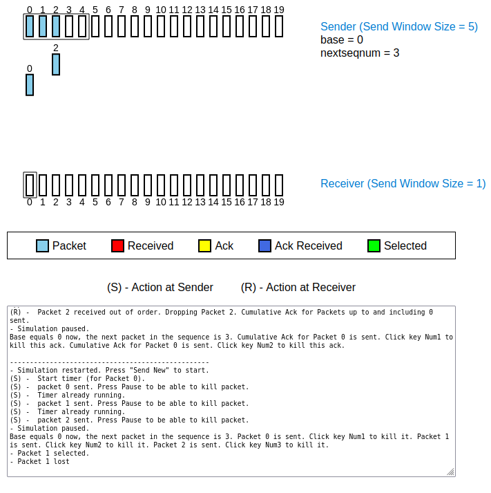
Figure 2: receiver seemingly sends an ACK for packet 2, but in actuality it is a duplicate ACK post_ACK

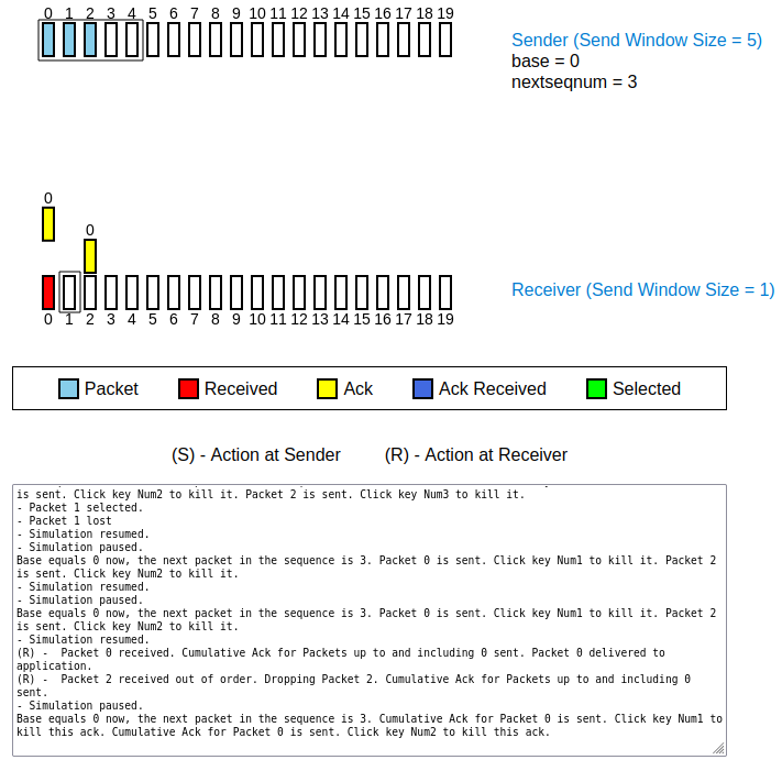
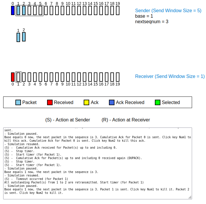
Figure 3: window slides one position further cum_ACK

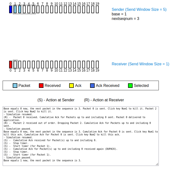
Figure 4: after the timeout for the lost packet 1 post_cum_ACK

GBN vs. TCP

GBN protocol incorporates almost all of the techniques used in TCP:
- sequence numbers
- cumulative acknowledgments
- checksums
- timeout/retransmit operation

Selective Repeat

just play with Kurose animations:
- SR
- e.g. send 3 packets, kill packet 1 and wait for the timeout and see what happens

Sender

as before, window of N consecutive sequence numbers
as before, window can only be advanced when the lowest sequence number in it is ACKed
- it may need to be advanced multiple values, if other packets have been ACKed out-of-order
individual timer for every packet that it sends
individual timeout/retransmit

receiver

individual ACKs for each received packet
- i.e. no duplicate ACKs: out-of-order packets are ACKed like in-order packets!
out-of-order buffer: packets are buffered for eventual in-order delivery to upper layer
- i.e. multiple packets together may be delivered to the upper layer, if out-of-order packets have been received by the receiver (whereas for GBN only one packet at a time is delivered)

Dilemma

watch: Kenan Casey, chapter 3.4, 57:20

SRDilemma

While the packet 0 arriving is a duplicate, the receiver will treat it as new data and deliver this duplicate up to the application out-of-order! The receiver is “blind” to the state of the sender except that it can infer through the control messaging.
- problem: The reliable transfer protocol must guarantee in-order delivery!
solution: window size must be $\leq$ half the size of the sequence number space

TCP

watch: Kurose
phth: mostly like GBN; K. Casey: mixture of both GBN and SR
unicast (aka point-to-point aka one-to-one communication, i.e. one sender and one receiver)
in-order byte stream (abstraction)
- i.e. there are no “message boundaries”, it is just a stream of bytes that can flow in either direction
connection-oriented
- i.e. there is a handshaking setup process
  - state variables
  - buffers
  - overhead associated with setting up the connection
full duplex data
- bi-directional data flow in same connection
- MSS: maximum segment size
  - Wireshark: there is an MSS= in the [SYN] packet “Info” column or [SYN, ACK] packet “Info” column
cumulative ACKs
- the sender assumes that this ACK with sequence number $n$ indicates that all packets with a sequence number up to and including $n$ have been correctly received at the receiver (therefore “cumulative”)
pipelining
- better utilization of the network
- TCP congestion and flow control set window size
flow controlled
- sender will not overwhelm receiver

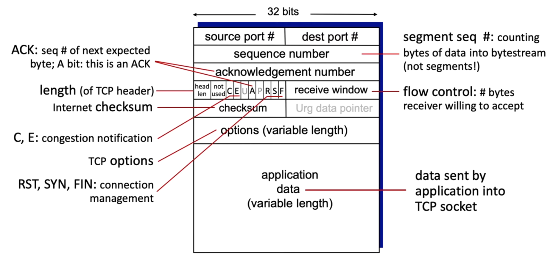
TCP Segment Format

“TCP options” field can have a variable length, and therefore, a “TCP header length” field is needed
Grey fields (URG for “urgent data”, PSH for “push data now”) are not really used, in practice

Seq and ACK Fields

sequence number field: byte stream “number” of the first byte in that segment’s payload data
ACK field: sequence number of next byte expected from other side (holds for both sides, receiver and sender! See Figure 6.)
cumulative ACKs (cf. section GBN sender)

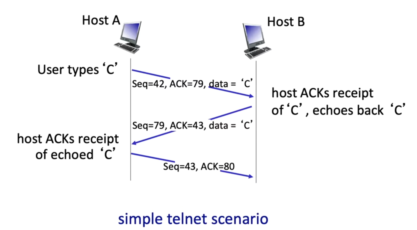
Figure 5: Seq and ACK fields

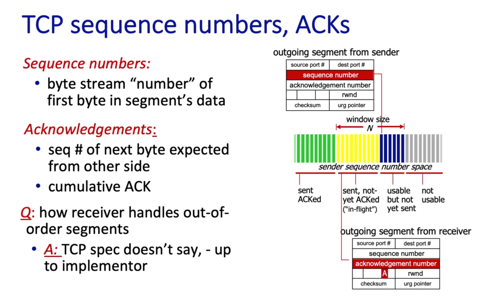
Figure 6: Note: resent ACK is always one more than the received Seq that triggered this ACK!

RTT and timeout

too short: unnecessary retransmission
too long: long timeout
estimate RTT:
- SampleRTT: measured time from segment transmission until ACK receipt
- EstimatedRTT $= (1 - \alpha) \times$ EstimatedRTT $+ \alpha \times$ SampleRTT (typically: $\alpha = 0.125$)
- DevRTT $= (1 - \beta) \times$ DevRTT $+ \beta \times |$ SampleRTT $-$ EstimatedRTT $|$
- TimeoutInterval $=$ EstimatedRTT $+ 4 \times$ DevRTT

Sender

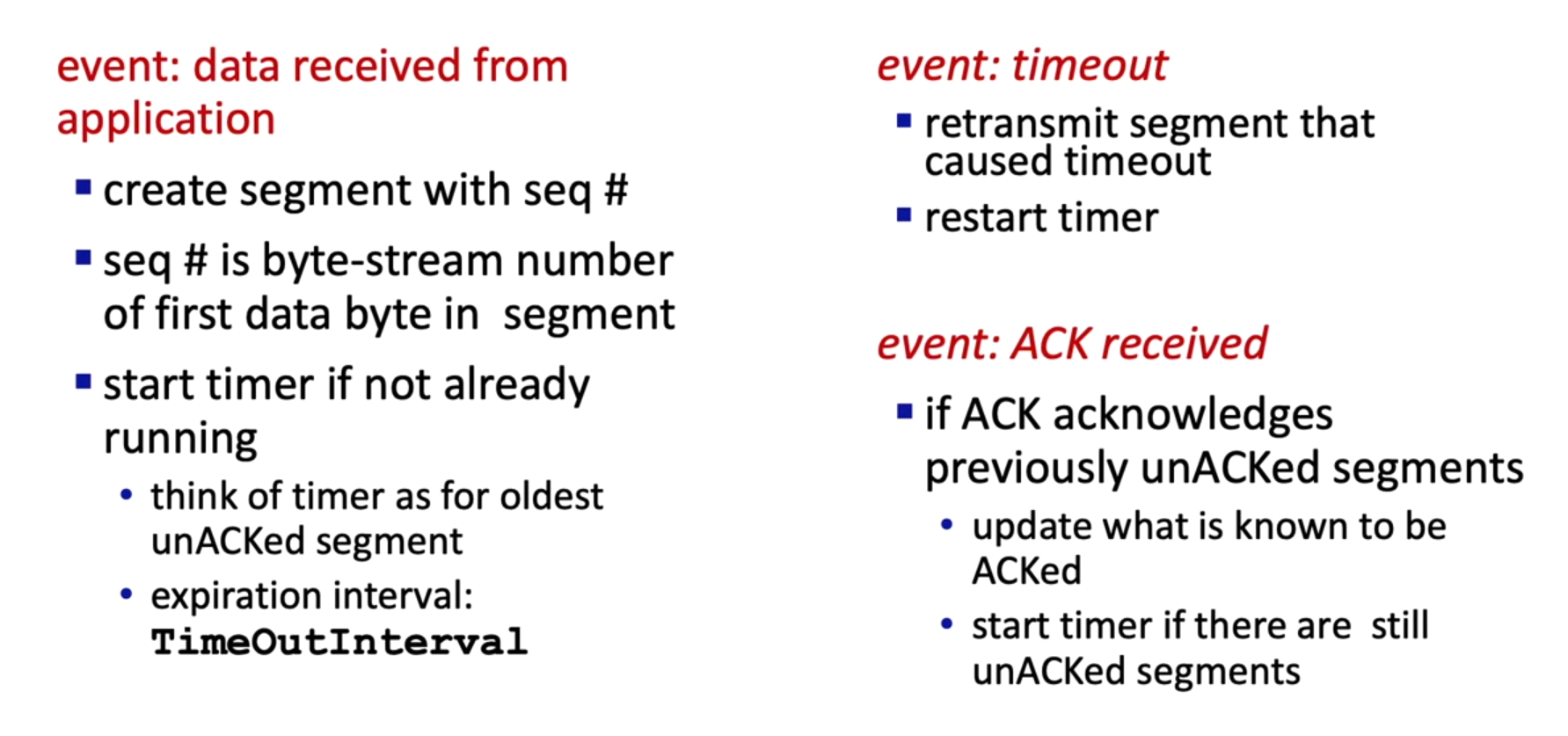
Receiver

watch: Kurose example scenarios

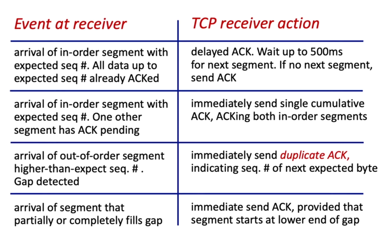
Fast Retransmit

fast retransmit: resend unACKed segment with smallest Seq when three duplicate ACKs are received
- three duplicate ACKs = segment following the segment that has been ACKed three times has been lost
- Wireshark: watch
  - after getting three [TCP Dup ACK] from the receiver (3 [TCP Dup ACK] = receiver says to the sender “something went missing” → packet loss), the sender triggers a [TCP Fast Retransmission]
  - after the 3 [TCP Dup ACK] packets and the [TCP Fast Retransmission] packet there will be a lot of other [TCP Dup ACK]. They are for all the other packets that arrived, but should have arrived actually after the lost packet.
  - filter by tcp.analysis.flags to quickly jump to [TCP Dup ACK] and [TCP Fast Retransmission] packets (black packets in the “Packet List” pane)
  - after a Fast Retransmit the cwnd will be reset to a small MSS number and will build up again (see video)
    - the build up speed depends on the used algorithm (e.g. in TCP Slow Start cwnd will grow exponentially)

TCP Implementation

KR238: RFC recommended TCP timer implementations use only a single retransmission timer, even if there are multiple transmitted but not yet acknowledged segments
- because timer management can require considerable overhead
duplicate ACKs instead of NAKs

Is TCP a GBN or an SR protocol?

From KR book.

TCP (without SACKs) looks a lot like a GBN-style protocol
differences:
1. Many TCP implementations will buffer correctly received but out-of-order segments
2. When N packets are sent and arrive, but the ACK for one of these packets (not the last one!) gets lost.
  - GBN would retransmit this packet and all following packets.
  - TCP would only retransmit the packet for which the ACK was lost.
TCP with SACKs and selective retransmissions looks a lot like SR protocol
- SACK: selective acknowledgment, acknowledge out-of-order segments selectively
  - Wireshark: to see if SACKs are enabled look if there is a SACK_PERM=1 in the [SYN] packet “Info” column or [SYN, ACK] packet “Info” column
  - watch
- selective retransmission: skipping the retransmission of segments that have already been selectively acknowledged
Thus, TCP is a hybrid of GBN and SR protocols

Flow Control

watch: K. Casey
speed-matching service

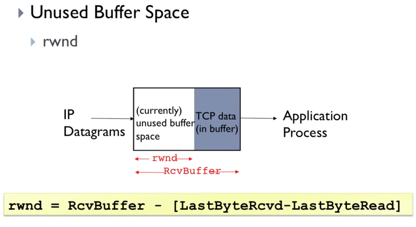
RcvBuffer: used and unused buffer space (in bytes)
rwnd: unused buffer space (in Wireshark: Window size value)

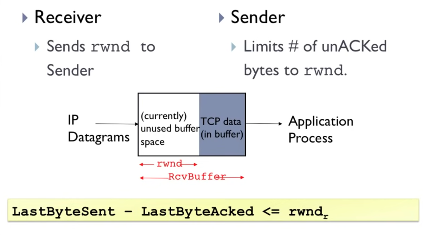
Implementation

receiver: every ACK contains an rwnd field
sender limits the number of unACKed bytes ($= ($LastByteSent $-$ LastByteAcked$)$, see yellow bars in Figure 5) to the size of the rwnd
- Wireshark: watch

Connection Management: Three-Way Handshake

Establish a connection

SYN segment, SYNACK segment, ACK segment
SYN packet
- the client sends a SYN packet to the server
- Seq field is set to: client randomly chooses an initial sequence number client_isn
- does not contain any data
- SYN bit is set to 1
SYN-ACK packet
- the server responds with a SYN-ACK packet
- Seq field is set to: server randomly chooses its own initial sequence number server_isn
- the server allocates buffers and variables to the connection (see SYN Flood Attack)
- does not contain any data
- SYN bit is set to 1
- ACK field is set to client_isn + 1
ACK packet
- the client saying “I am accepting your connection and starting the TCP connection”
- Seq field is set to client_isn + 1
- the client allocates buffers and variables to the connection
- may contain data
- SYN bit is set to zero
- ACK field is set to server_isn + 1
In each future segment, the SYN bit will be set to zero

SYN Flood Attack

SYN Flood Attack
- solution: SYN Cookies
  - don’t allocate “resources” (i.e. buffers and variables) until ACK (3rd handshake step) received (confirming that there is really a client out there)

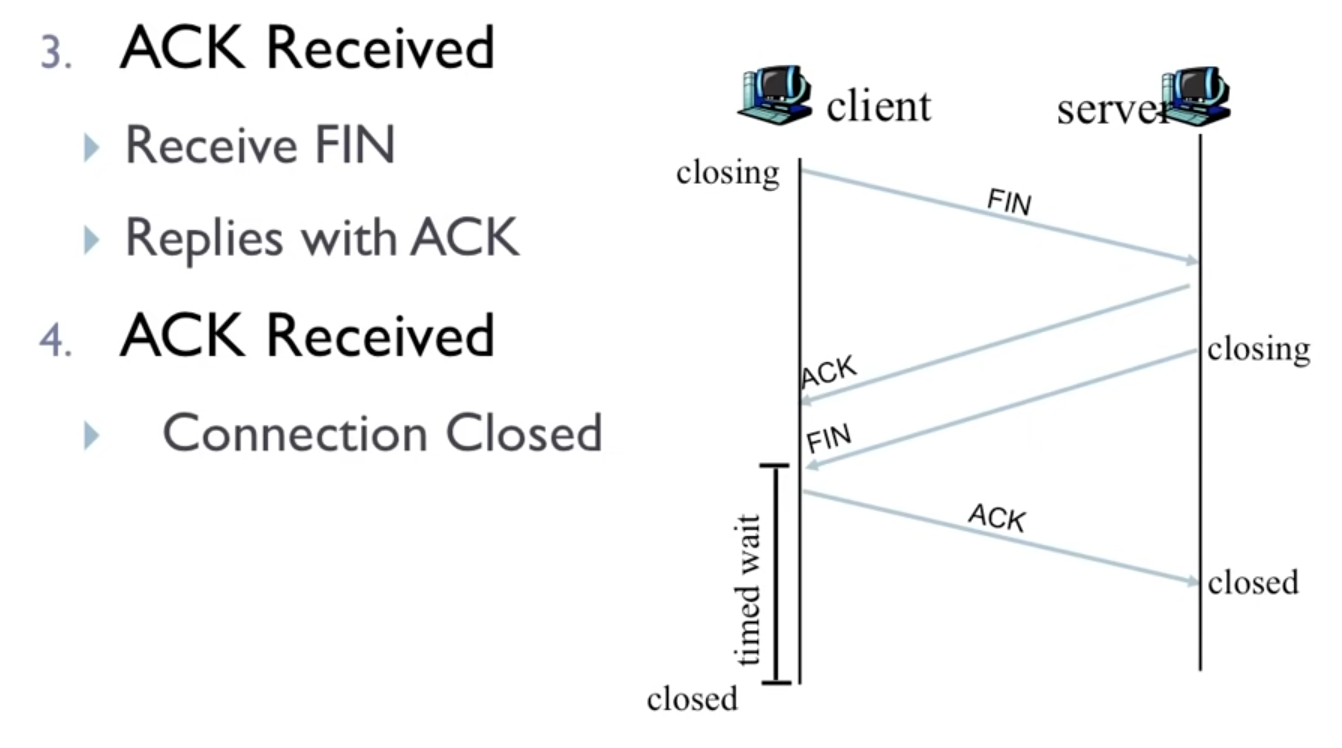
Close a connection

4-step process: FIN, ACK, FIN, ACK
- after the last ACK all resources in both hosts are deallocated
shutdown/FIN segment: FIN bit set to 1
timed wait: “lets the TCP client resend the final acknowledgment in case the ACK is lost”
- time is implementation-dependent: typically 30 sec, 1 min or 2 min

Reset Segment

segment that has its RST flag bit set to 1
event: when a host receives a TCP segment whose port numbers or source IP address do not match with any of the ongoing sockets in the host
action: send a reset segment to the source
- when a host sends a reset segment, it is telling the source “I don’t have a socket for that segment. Please do not resend the segment.”

Not covered

pathological scenarios, for example, when both sides of a connection want to initiate or shut down at the same time

nmap

port scanner
“case the joint” for
- open TCP ports,
- open UDP ports,
- firewalls and their configurations,
- versions of applications and operating systems
most of this is done by manipulating TCP connection-management segments.
source: KR p.192 “Port Scanning”:
- For TCP, nmap sequentially scans ports, looking for ports that are accepting TCP connections.
- For UDP, nmap again sequentially scans ports, looking for UDP ports that respond to transmitted UDP segments.
- In both cases, nmap returns a list of open, closed, or unreachable ports.
- useful for system administrators, who are often interested in knowing which network applications are running on the hosts in their networks.
- useful for attackers, in order to “case the joint” (i.e. checking which ports are open on target hosts)
  - now, IF an application has a known security flaw and is listening on an open port, THEN a remote user can execute arbitrary code on the vulnerable host!
    - e.g. Slammer worm
to explore port portnumber nmap sends a TCP SYN segment with destination port portnumber
3 possible outcomes
- SYNACK
  - target host is running an application with TCP port portnumber
  - nmap returns open
- RST
  - target host is not running an application with TCP port portnumber
  - attacker at least knows that port portnumber is not blocked by any firewall
- nothing
  - SYN segment was blocked by a firewall

Congestion Control

watch: Kurose
revisit KR chapter 1.4 “Delay, Loss” (in particular, Figure 1.18 “Dependence of average queuing delay on traffic intensity”)
key takeaways (phth):
- it’s not all about maximizing throughput, but it’s also about minimizing delay! Throughput and delay must be considered together!
  - Delay (includes e.g. queueing delay) can be measured via RTT (traceroute)
  - Throughput can be measured
problems of congestion
- we lose packets (because buffers overflow, so that there is not enough room to store packets, see chapter 1.4 “Delay, Loss” K. Casey)
- long delays (because of the queueing in the routers)

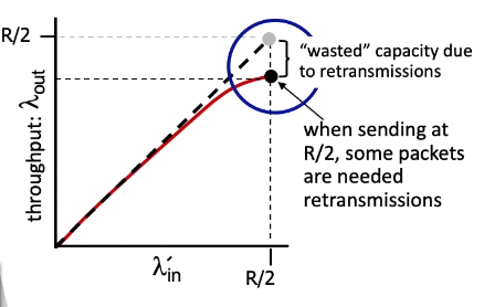
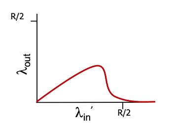
Figure 7: 2 connections (red line and blue line) are shared over a single hop, i.e. if the full link capacity is R each connection’s throughput is limited to at most R/2

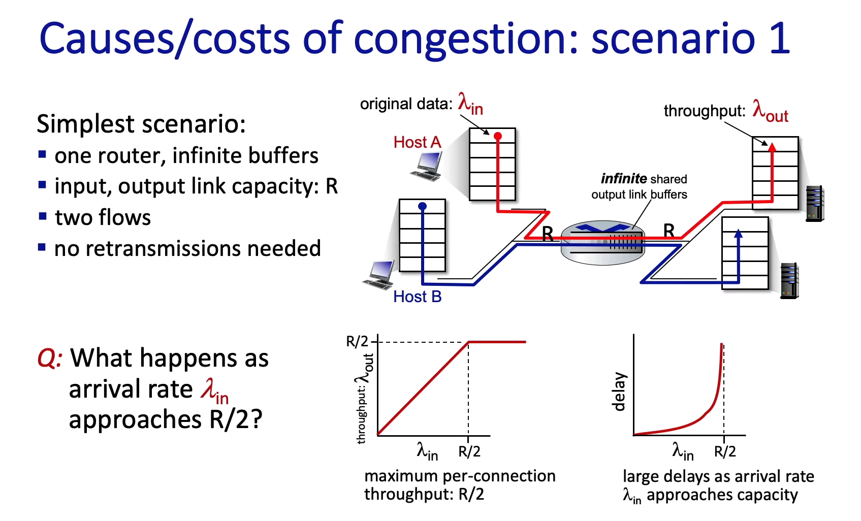
note about Figure 7: the senders may send at a rate higher than R/2 (because of the infinite buffer [= storage]), but the output rate $\lambda$ will not increase any further
- Kurose video:
  - “if each sender would be sending at a rate faster than R/2 the throughput would simply max out at R/2 per flow” (deshalb der Knick im Graph)
  - “that’s because the router’s input and output links cannot carry more than R bps of traffic, R/2 for each of the two flows”
  - read KR 1.4 “Delay, Loss”
note about Figure 7: unlimited buffer, thus, queueing delay can go to infinity (for a limited buffer size the delay does not really approach infinity, instead packets will be dropped, see KR 1.4.2 “Packet loss”)

Costs of Congestion

watch: Kurose
scenario 1: Large queueing delays are experienced as the packet arrival rate approaches the link capacity.
scenario 2a: packet loss: sender must perform retransmissions in order to compensate for dropped (lost) packets due to buffer overflow

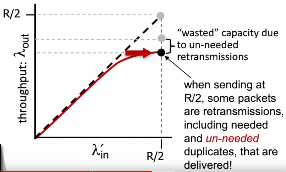
scenario 2b: premature time out of the sender: unneeded retransmissions by the sender in the face of large delays may cause a router to use its link bandwidth to forward unneeded copies of a packet

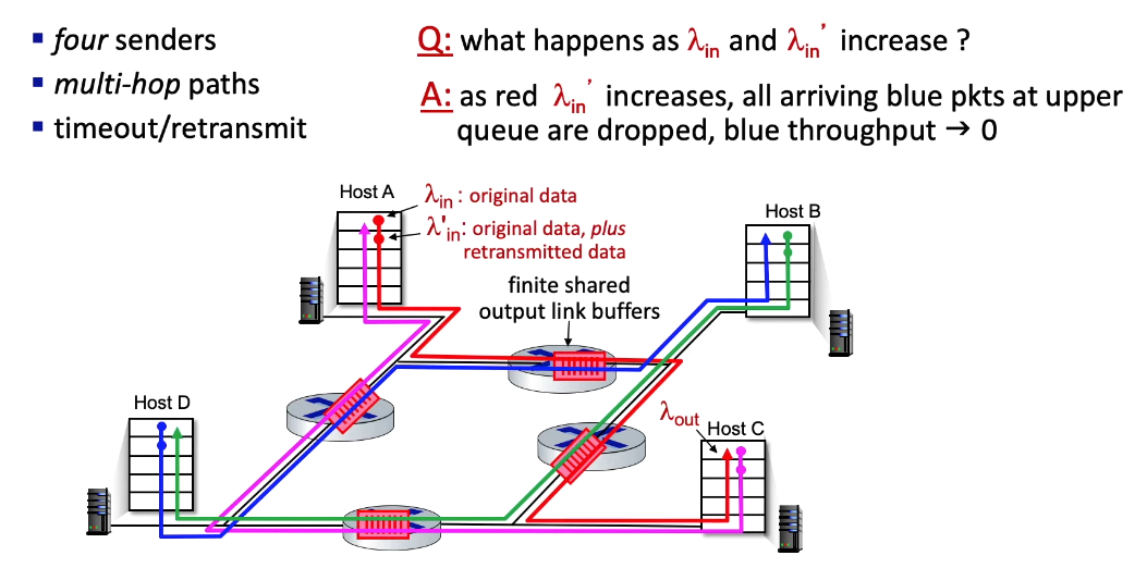
scenario 3: multiple hops:
- when e.g. $\lambda_{in}’ \rightarrow \frac{R}{2}$ for the red flow, then this first hop traffic will crowd out the second hop traffic and eventually all other upstream routers, too
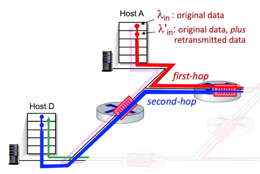
- when a packet is dropped along a path, the transmission capacity that was used at each of the upstream links to forward that packet to the point at which it is dropped ends up having been wasted
- “congestion collaps” phenomenon

Approaches

End-to-end congestion control
- required for TCP
- presence of network congestion must be inferred by the end systems based only on observed network behavior (for example, via packet loss and delay)
- this is what default TCP does
  - TCP segment loss as indication of network congestion (decreases window size accordingly)
  - increased round-trip segment delay as indicator
Network-assisted congestion control
- optional for TCP
  - more recently, IP and TCP may also optionally implement network-assisted congestion control
- routers provide explicit feedback to the sender and/or receiver regarding the congestion state
- two ways
  - (1) direct feedback from router to the sender via “choke packet”
  - (2) feedback from receiver to the sender (more common than (1)): Router marks/updates a field in a packet flowing from sender to receiver. When the receiver gets this marked packet the receiver notifies the sender of the congestion, so the sender can slow down. (Thus, this method takes a full RTT!)

TCP Congestion Control

Loss based approaches

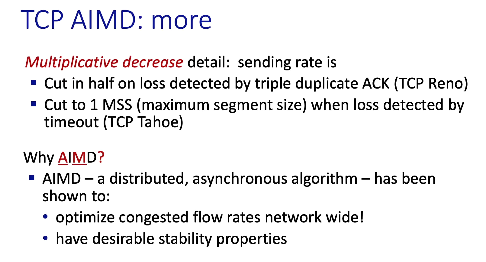
AIMD

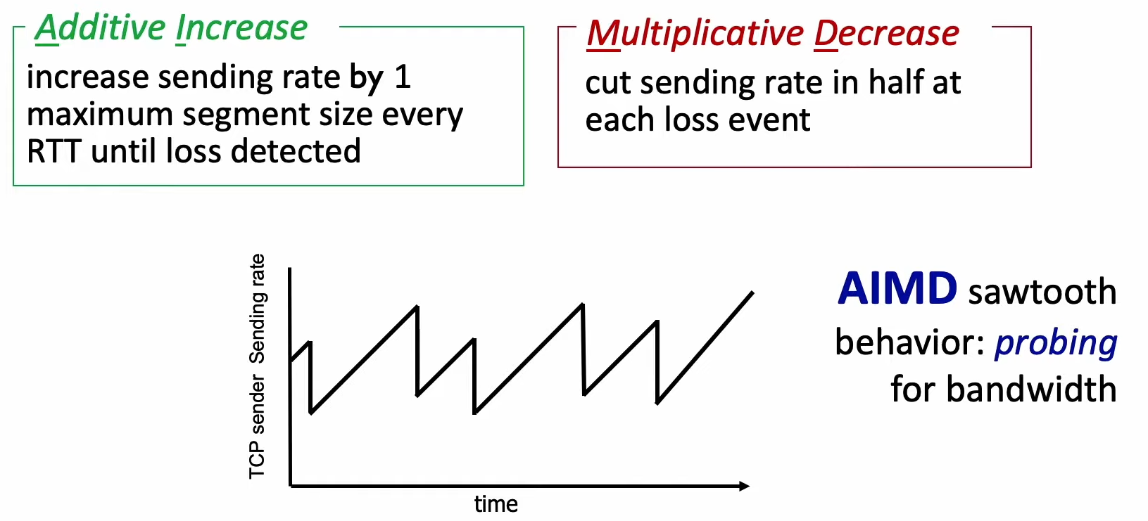
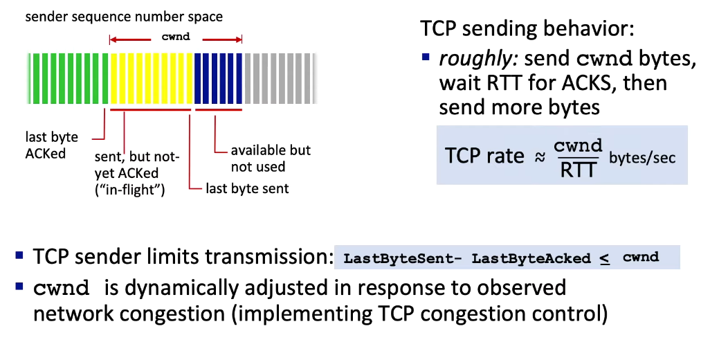
“Thus the sender’s send rate is roughly cwnd/RTT bytes/sec. By adjusting the value of cwnd, the sender can therefore adjust the rate at which it sends data into its connection.” (KR 3.7.1)

cwnd: congestion window
- internal parameter of the sending machine, not directly visible in Wireshark!
Wireshark:
- watch
- see in this packetlife post

More precisely:

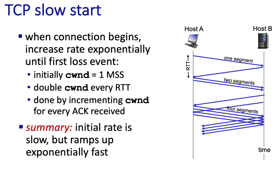
Slow Start

Wireshark:

see in this packetlife post
see in this networkers-online.com post

Transition: From Slow Start to AIMD

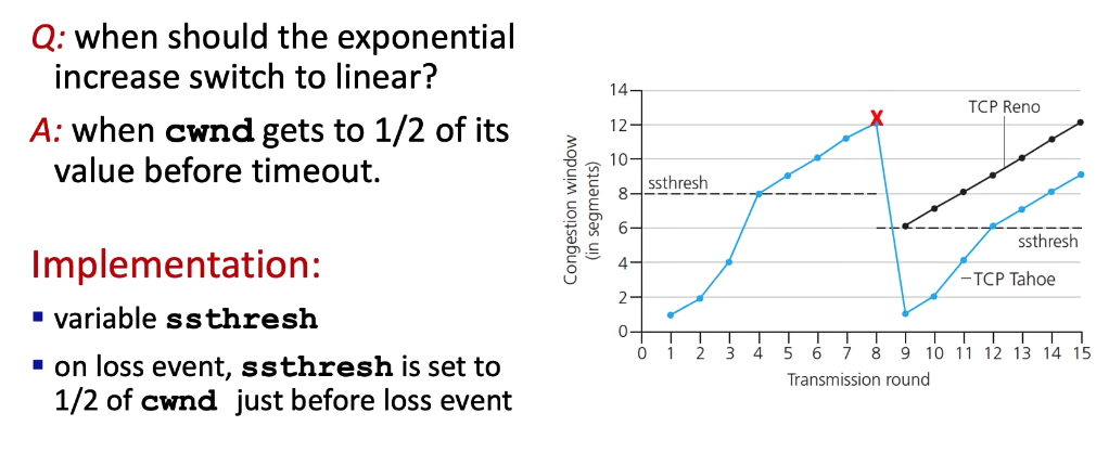
ssthresh: slow start threshold (internal parameter of the sending machine, not directly visible in Wireshark!)
Wireshark: watch
- either the rwnd makes the sender “pull the break”
- or the network cannot handle as much data as the sender is putting out there on the wire (see Fast Retransmit)
see also Wireshark TCP Lab “congestion window” estimate task

TCP CUBIC

one of the most notable modifications to the original TCP

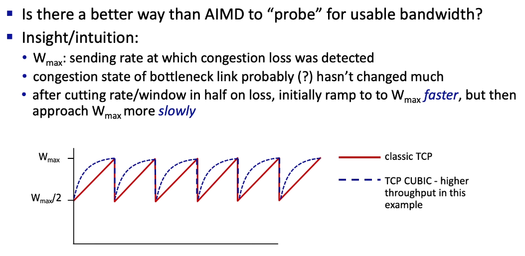
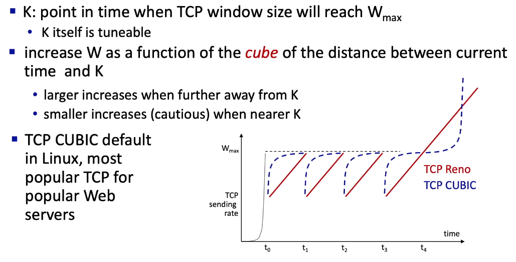
among the 5000 most popular web servers nearly 50% of them run a version of TCP CUBIC

Delay based approaches

based on using RTT measurements (recall RTT measurement)

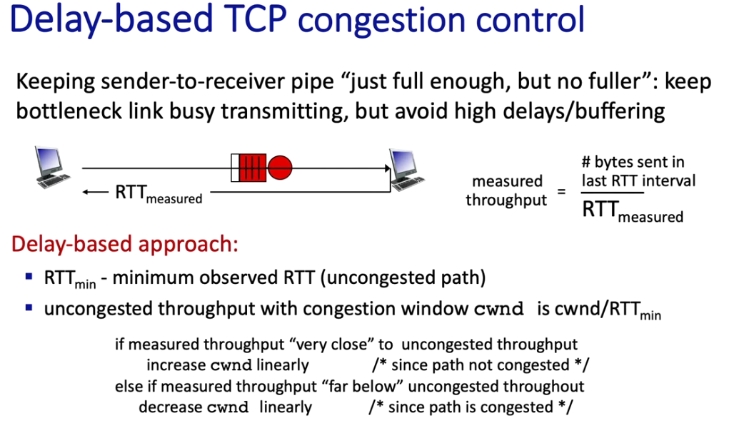
Note: cwnd $\propto$ sender’s send rate - the sender controls his speed by setting cwnd

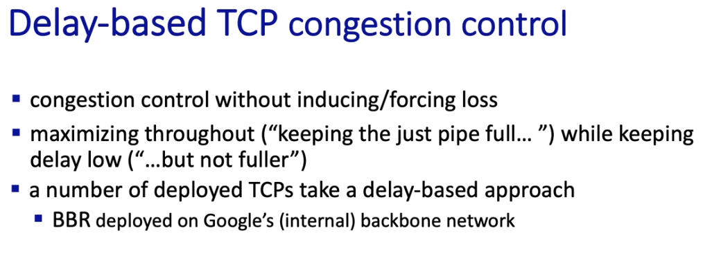
BBR: “Bottleneck Bandwidth and Round-trip propagation time”
- used for tcp traffic on Google’s internal network that interconnects its datacenters
- replaced CUBIC
- also deployed on Google and Youtube web servers

Network assisted approaches

ECN

“Explicit Congestion Notification”
router “in between” sets two bits in IP header
- more precisely: 2 bits of the 8-bit ToS field (“type of service” field) in the IP header (IPv6 header)
receiver sets ECE (Explicit Congestion Notification Echo) bit on ACK segment
- more precisely: C bit and E bit in the TCP header
from book: “The TCP sender, in turn, reacts to an ACK with a congestion indication by halving the congestion window, as it would react to a lost segment using fast retransmit, and sets the CWR (Congestion Window Reduced) bit in the header of the next transmitted TCP sender-to-receiver segment.”

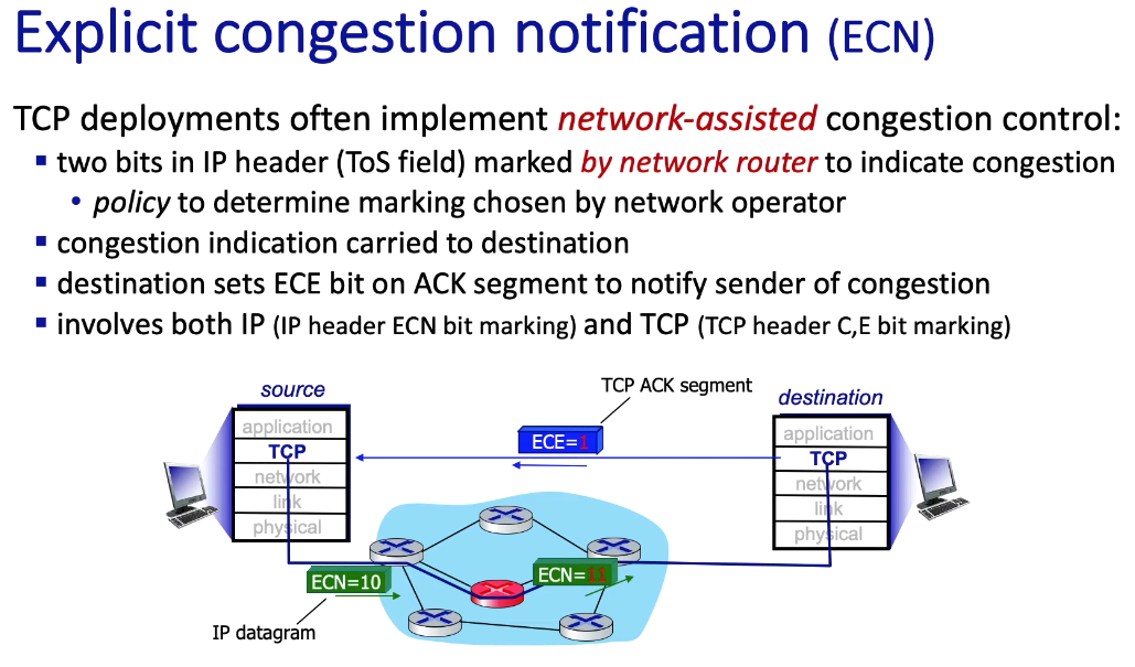
Note: “chosen by operator” means there is no standardized method in the RFC’s for how to set the ECN and ECE bits - from book: “RFC 3168 does not provide a definition of when a router is congested; that decision is a configuration choice made possible by the router vendor, and decided by the network operator.”

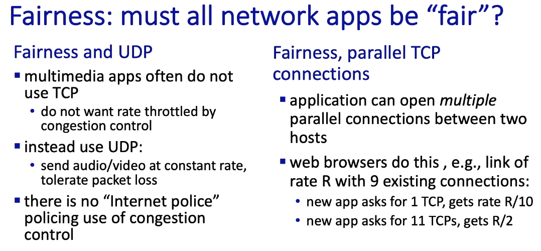
TCP Fairness

TCP is fair in the idealized scenario below, where only two connections (TCP sessions) are competing for throughput
- “fixed number of sessions”: i.e. there is no other connection
- “only in congestion avoidance”: (the bullet point is missing here probably) i.e. the router is always operating in congestion-avoidance mode

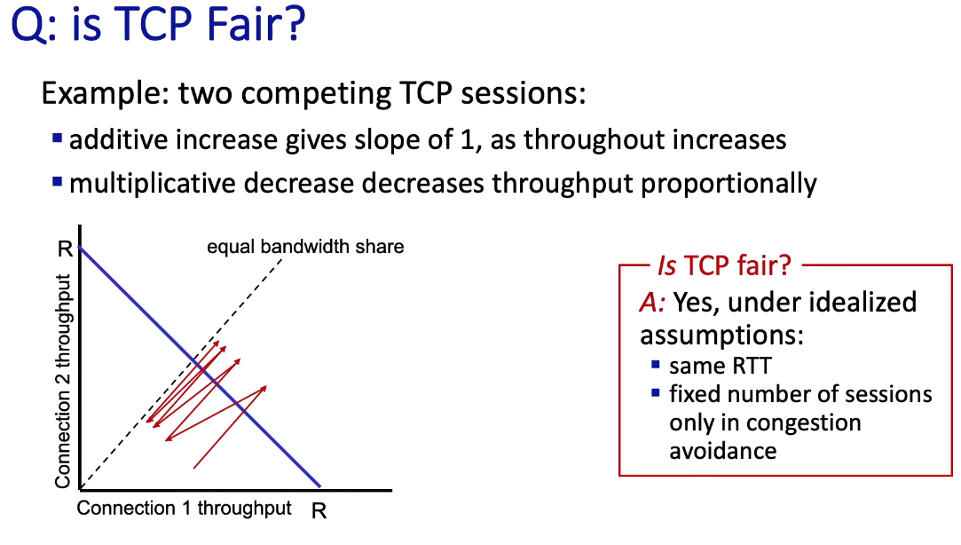
some web servers open up multiple parallel TCP connections allowing the web application to get more throughput than if it had just opened one connection

Share on

Twitter Facebook LinkedIn

DatKom Notes

Concepts

What every CS major should know

Networking

Specific recommendations

Recommended reading

Security

Specific recommendations

Recommended reading

Cryptography

Specific recommendations

Recommended reading

Linux commands

Basics

Tools

configuration

MTU, MSS

Segmentation Offload

ports, firewall

Measurements

Throughput testing (iperf3)

tshark

Get the Field Name

Examples

Wireshark

Must-Knows

Wireshark GUI meaning

The “Packet List” Pane

TCP

RTT Graph

Time-Sequence-Graph (Stevens)

Time-Sequence-Graph (tcptrace)

“Window Scaling” Graph

Measure Throughput

Fields

OSI Model

Multiplexing

Circuit Switching (TDM or FDM)

Packet Switching (statistical multiplexing)

The Internet

Tiers of networks

Delay and Loss

Queueing Delay

Application layer (Brief)

Transport layer (Brief)

Transport protocols: TCP/UDP

Application Layer (Layer 7)

Web and HTTP

WebSocket

Email

SMTP

DNS

Recursive vs Iterative DNS query

DNS Cache

DNS Cache in Ubuntu, Time to Live (TTL)

DNS Resource Records (RRs)

nslookup, dig

ip, ifconfig, ipconfig, nmcli, iwconfig

Loopback address, Localhost

P2P File Distribution

RTSP, WebRTC

Transport Layer (Layer 4)

TCP and UDP

TCP

UDP

Multiplexing/Demultiplexing

Segments, Datagrams, Messages (Encapsulation)

Payload

Demultiplexing

Checksum

Ones’ Complement

Two’s Complement

Endianness

End-to-End Principle

Principles of Reliable Data Transfer

Sequence Numbers

Utilization

Pipelining

Go-Back-N (sliding-window protocol)

Sender