CNN Concept

Good Overviews

Wikipedia

Why do CNNs work?

Sparse Connectivity

as opposed to Full Connectivity
Goodfellow_2016:
- Convolutional networks, however, typically have sparse interactions (also referred to as sparse connectivity or sparse weights). This is accomplished by making the kernel smaller than the input.
  - This means that we need to store fewer parameters, which both
    - reduces the memory requirements of the model and
    - improves its statistical efficiency.
  - It also means that computing the output requires fewer operations.
  - These improvements in efficiency are usually quite large.

Note: increases bias of the model, but not the variance
Goodfellow_2016:
- The parameter sharing used by the convolution operation means that rather than learning a separate set of parameters for every location, we learn only one set.

Efficiency of the Convolution Operation

Goodfellow_2016:
- sparse connectivity and parameter sharing can dramatically improve the efficiency of a linear function for detecting edges in an image
  - [matrix multiplication vs convolution:]
    - Of course, most of the entries of the matrix would be zero. If we stored only the nonzero entries of the matrix, then both matrix multiplication and convolution would require the same number of floating point operations to compute.
    - Convolution is an extremely efficient way of describing transformations that apply the same linear transformation of a small, local region across the entire input.

achieved by convolution operation (aka “parameter sharing across locations”)
- Goodfellow_2016:
  - In the case of convolution, the particular form of parameter sharing causes the layer to have a property called equivariance to translation.
Goodfellow_2016:
- convolution creates a 2-D map of where certain features appear in the input. If we move the object in the input, its representation will move the same amount in the output.
- This is useful for when we know that some function of a small number of neighboring pixels is useful when applied to multiple input locations.
  - For example, when processing images, it is useful to detect edges in the first layer of a convolutional network. The same edges appear more or less everywhere in the image, so it is practical to share parameters across the entire image.
- [Caveat:] In some cases, we may not wish to share parameters across the entire image.
  - For example, if we are processing images that are cropped to be centered on an individual’s face, we probably want to extract different features at different locations—the part of the network processing the top of the face needs to look for eyebrows, while the part of the network processing the bottom of the face needs to look for a chin.
- Convolution is not naturally equivariant to some other transformations, such as changes in the scale or rotation of an image. Other mechanisms are necessary for handling these kinds of transformations.
source:
- because the convolution operator commutes wrt translation
source:
- Translational Equivariance or just equivariance is a very important property of the convolutional neural networks where the position of the object in the image should not be fixed in order for it to be detected by the CNN. This simply means that if the input changes, the output also changes. To be precise, a function $f(x)$ is said to be equivariant to a function g if $f(g(x)) = g(f(x))$.
Wiki: Equivariant Map
- That is, applying a symmetry transformation and then computing the function produces the same result as computing the function and then applying the transformation.

Reduction in Flexibility of Model

source:
- This [translational equivariance] means that translating the input to a convolutional layer will result in translating the output.
- [“flexibility reduction is good” and this is also why CNNs work well]:
  - There is a downside to complete flexibility. While we know that we can learn our target function, there’s also a whole universe of incorrect functions that look exactly the same on our training data. If we’re totally flexible, our model could learn any one of these functions, and once we move away from the training data, we might fail to generalise. For this reason, it’s often desirable to restrict our flexibility a little. If we can identify a smaller class of functions which still contains our target, and build an architecture which only learns functions in this class, we rule out many wrong answers while still allowing our model enough flexibility to learn the right answer. This might make a big difference to the necessary amount of training data or, given the same training data, make the difference between a highly successful model and one that performs very poorly.
  - A famous success story for this reduction in flexibility is the CNN. The convolutional structure of the CNN encodes the translation symmetries of image data. We’ve given up total flexibility and can no longer learn functions which lack translation symmetry, but we don’t lose any useful flexibility, because we know that our target function does have translation symmetry. In return, we have a much smaller universe of functions to explore, and we’ve reduced the number of parameters that we need to train.

Extend this idea

take this idea further: extending translation equivariance of CNNs to further symmetry classes $\Rightarrow$ “Group Equivariant CNNs” [Cohen, Welling 2016]

Translational invariance (via Pooling)

achieved by pooling operation
Goodfellow_2016:
- popular pooling functions include
  - the average of a rectangular neighborhood,
  - the L2 norm of a rectangular neighborhood, or
  - a weighted average based on the distance from the central pixel.
Goodfellow_2016:
- pooling helps to make the representation become approximately invariant to small translations of the input.
- Invariance to translation means that if we translate the input by a small amount, the values of most of the pooled outputs do not change.
- Invariance to local translation can be a very useful property if we care more about whether some feature is present than exactly where it is.
  - For example, when determining whether an image contains a face, we need not know the location of the eyes with pixel-perfect accuracy, we just need to know that there is an eye on the left side of the face and an eye on the right side of the face.
- [Caveat:] In other contexts, it is more important to preserve the location of a feature.
  - For example, if we want to find a corner defined by two edges meeting at a specific orientation, we need to preserve the location of the edges well enough to test whether they meet.
- The use of pooling can be viewed as adding an infinitely strong prior that the function the layer learns must be invariant to small translations. When this assumption is correct, it can greatly improve the statistical efficiency of the network.

Pooling

How to set size of pools?

larger pooling region $\Rightarrow$ more invariant to translation, but poorer generalization
- notice, units in the deeper layers may indirectly interact with a larger portion of the input
in practice, best to pool slowly (via few stacks of conv-pooling layers)
Mouton, Myburgh, Davel 2020:
- CNNs are not invariant to translation! Reason:
  - This lack of invariance is attributed to
    - the use of stride which subsamples the input, resulting in a loss of information,
    - and fully connected layers which lack spatial reasoning.
- “local homogeneity” (dataset-specific characteristic):
  - determines relationship between pooling kernel size and stride required for translation invariance

Learning Invariance to other Transformations

Goodfellow_2016:
- [pooling over different filters (instead of pooling spatially over the image) allows learning rotation invariance] Pooling over spatial regions produces invariance to translation, but if we pool over the outputs of separately parametrized convolutions [i.e. different filters], the features can learn which transformations to become invariant to (see figure 9.9).
  - This principle is leveraged by maxout networks (Goodfellow et al., 2013a) and other convolutional networks.

Strided Pooling

Goodfellow_2016:
- [advantages of strided pooling] Because pooling summarizes the responses over a whole neighborhood, it is possible to use fewer pooling units than detector units, by reporting summary statistics for pooling regions spaced $k$ pixels apart rather than $1$ pixel apart.
  - See figure 9.10 for an example.
  - This improves the computational efficiency of the network because the next layer has roughly $k$ times fewer inputs to process.
  - When the number of parameters in the next layer is a function of its input size (such as when the next layer is fully connected and based on matrix multiplication) this reduction in the input size can also result in improved statistical efficiency and reduced memory requirements for storing the parameters.
    - less parameters $\Rightarrow$ reduces overfitting

Nonlinear Downsampling Method

Goodfellow_2016:
- [pooling as a nonlinear downsampling method for a following classification layer] For many tasks, pooling is essential for handling inputs of varying size.
  - For example, if we want to classify images of variable size, the input to the classification layer must have a fixed size.
    - This is usually accomplished by varying the size of an offset between pooling regions so that the classification layer always receives the same number of summary statistics regardless of the input size.
      - For example, the final pooling layer of the network may be defined to output four sets of summary statistics, one for each quadrant of an image, regardless of the image size.

Nonlinearities

What do ReLU layers accomplish ?

Piece-wise linear tiling: mapping is locally linear.
Montufar et al. “On the number of linear regions of DNNs” arXiv 2014
- ReLU layers do local linear approximation.
  - Number of planes grows exponentially with number of hidden units.
    - Multiple layers yield exponential savings in number of parameters (parameter sharing).

Other Reasons (Ranzato)

[source]

whyconvnetswork

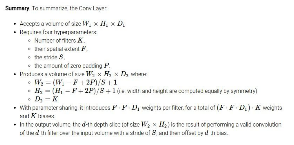
Conv Layer properties

key points:
- output size: $\text{Floor}(\frac{W-F+2P}{S}+1) \times \text{Floor}(\frac{H-F+2P}{S}+1) \times K$
- number of parameters: $(F\cdot F\cdot D_{input}+1)\cdot K$
  - Note: for FC layers: number of parameters: $(c \cdot p)+c$
    - where
      - current layer neurons $c$
      - previous layer neurons $p$
$\text{RF}i=(\text{RF}{i-1}-1)S_i+F_i$
- $F_i$: Kernel size
- $S_i$: Stride
Ranzato slides:
- computational cost per conv layer: $(F\cdot F\cdot D_{input}+1)\cdot (\frac{W-F+2P}{S}+1)\cdot (\frac{H-F+2P}{S}+1)\cdot K$
  - [das ist nicht “output size” mal “number of parameters”! Sonst wäre $K$ doppelt, weil $K$ in beiden enthalten ist!]
    - [cost für EINEN Kernel: $(F\cdot F\cdot D_{input}+1)\cdot (\frac{W-F+2P}{S}+1)\cdot (\frac{H-F+2P}{S}+1)$]

How many feature maps (per conv layer)?

Ranzato slides:
- Usually, there are more output feature maps than input feature maps.
- Convolutional layers can increase the number of hidden units by big factors (and are expensive to compute).

What’s the size of the filters?

The size of the filters has to match the size/scale of the patterns we want to detect (task dependent)
Why is the size of $F$ always an odd number?
- usually $1$, $3$, $5$, $7$ and sometimes $11$
- you can use filters with even numbers, but it is not common
- the lowest people use is $3$, mainly for convenience
  - you want to apply the filter around a well-defined position that “exists” in the input volume (see traditional image processing)

What’s the receptive field of a filter?

$\text{RF}i=(\text{RF}{i-1}-1)S_i+F_i$
- $F_i$: Kernel size
- $S_i$: Stride

Padding

Why pad with zeros ?

idea: you do not want the outer padded pixels to contribute to the dot product
- [well, this is engineering: i.e. if you have some reason to use other paddings, just try it]
but you can also use other padding techniques, but it is less common, in practice

VALID vs SAME padding

source
- The general meaning of SAME and VALID padding are:
  - SAME: Expects padding to be such that the input and output is of same size (provided stride=1) (pad value = kernel size)
  - VALID: Padding value is set to 0
- Note: SAME padding is different in different frameworks.

What’s the function of 1x1 filters?

Channel-wise pooling (aka cross-channel downsampling, cross-channel pooling)
- $\Rightarrow$ dimensionality reduction (in depth), while introducing nonlinearity

Data Augmentation

these methods introduce additional hyperparameters

Implementation

usually done in a separate CPU (or GPU) thread, so that training and augmentation can be done in parallel

Common examples

cropping
zooming
flipping
mirroring
Color PCA
- for each pixel an Eigenspace is computed that highlights the expected color variations and then within those color variations you can adjust the colors of the entire image
- AlexNet paper:
jittering
- ColorJitter is a type of image data augmentation where we randomly change the brightness, contrast and saturation of an image.
used less often, computationally expensive:
- rotation
- shearing
- local warping

Test-time augmentation (TTA)

apply cropping and flipping also at test time
ColorPCA at test time can improve accuracy another $1\%$, but runtime will increase!
My question: Is zooming at test time not necessary because CNNs are invariant to translations?
- convolutions are not naturally invariant to other transformations such as rotation and scale [zoom] (see above and Goodfellow_2016)
Does TTA make sense? Stanford exam
- Both answers are right.
- If no, then explain that we want to test on real data only.
- If yes, then explain in which situation doing data augmentation on test set might make sense (e.g. as an ensemble approach in image classifiers).

CNN Datasets

MNIST

There are 60,000 images in the training dataset and 10,000 images in the validation dataset, one class per digit so a total of 10 classes, with 7,000 images (6,000 train images and 1,000 test images) per class.

ImageNet Dataset vs PASCAL Dataset

PASCAL: classify “bird”, “cat”, … etc.
ImageNet: more finegrained classes:
- e.g.
  - instead of “bird” you have to classify “flamingo”, “cock”, “ruffed grouse”, “quail”, … etc.
  - instead of “cat” you have to classify “Egyptian cat”, “Persian cat”, “Siamese cat”, “tabby”, … etc.

CNN Architectures

AlexNet vs LeNet

architecture:
- conv
- ReLU
- normalization (local response normalization)
- max pool
- conv
- ReLU
- normalization
- max pool
- a few more conv layers with ReLU,
- max pool (after 5. conv)
- several FC layers with ReLU
similar to LeNet
AlexNet has more layers
60 million parameters
first use of ReLU
local response normalization layers (not used anymore)
Dropout
GPU acceleration (CUDA Kernel by Krizhevsky)
more data
Momentum
learning rate reduction (divide by 10 on plateaus)
- paper:
  - […] divide the learning rate by 10 when the validation error rate stopped improving with the current learning rate. The learning rate was initialized at 0.01 and reduced three times prior to termination […]
ensembling
weight decay
- paper:
  - We trained our models using stochastic gradient descent with a batch size of 128 examples, momentum of 0.9, and weight decay of 0.0005. We found that this small amount of weight decay was important for the model to learn. In other words, weight decay here is not merely a regularizer: it reduces the model’s training error.
efficient data augmentation
1. image translations and horizontal reflections
2. Color PCA
  - We employ two distinct forms of data augmentation, both of which allow transformed images to be produced from the original images with very little computation, so the transformed images do not need to be stored on disk. In our implementation, the transformed images are generated in Python code on the CPU while the GPU is training on the previous batch of images. So these data augmentation schemes are, in effect, computationally free
  - [i.e. no additional memory, only little additional computation].

ZFNet vs AlexNet

Zeiler, Fergus
basically, same idea
better hyperparameters, e.g.
- different stride size
- different numbers of filters
source:
- ZFNet is a classic convolutional neural network. The design was motivated by visualizing intermediate feature layers and the operation of the classifier. Compared to AlexNet, the filter sizes are reduced and the stride of the convolutions are reduced.

VGGNet vs AlexNet

Simonyan, Zisserman (Oxford)
mainly used: VGG16 and VGG19
deeper with smaller filters
- $3\times 3$ filters all the way
  - (1) deeper (3 layers instead of 1),
  - (2) more nonlinearities and
  - (3) fewer parameters for same effective receptive field
higher total memory usage (most memory in early layers)
- need to store numbers (e.g. activations) during forward pass because you will need them during backprop
roughly twice as many parameters (most parameters in later FC layers)
try to maintain a constant level of compute through layers [Leibe Part 17 Folie 23: “same complexity per layer”]:
- downsample spatially and simultaneously increase depth as you go deeper
  - Leibe:
    - Heuristic: double the $\text{#}(\text{filter channels})$ whenever pooling halves the dimensions
      - saves computation by working on smaller input
similar training procedure as AlexNet
no local response normalization
ensembling (like AlexNet)

GoogleNet vs AlexNet

Christian Szegedy, Dragomir Anguelov
deeper
- 22 layers
  - [inception module zählt als 2 layer, ansonsten zähle alle Conv layer; zähle sozusagen alle “blauen Kästchen”]
computationally more efficient (because no FC layers)
no FC layers (except for one for the classifier)
- fewer parameters (12x less than AlexNet)
- computationally more efficient
use of “local network topology” aka “network within a network” aka inception module
- idea: filters with different sizes, will handle better multiple object scales
- applying several different kinds of filter operations in parallel
  - 1x1,
  - 3x3,
  - 5x5,
  - 3x3 max pooling (to summarize the content of the previous layer)
    - Note: this max pooling layer uses SAME padding (i.e. input size=output size), so that the concatenation with the other outputs is possible
- concatenate all outputs depth-wise
use of bottleneck layers aka “one-by-one convolutions”
- project feature maps to lower (depth) dimension before convolutional operations
- compared to an inception module without bottleneck layers:
  - reduces total number of ops (i.e. computational complexity)
  - prevents depth from blowing up after each inception module
  - less parameters
  - more nonlinearities
architecture:
- stem network (similar to AlexNet)
  - Conv - MaxPool - LocalRespNorm - Conv - Conv - LocalRespNorm - MaxPool
- 9 inception modules all stacked on top of each other
- extra stems
  - auxiliary classification outputs for training the lower layers
    - inject additional gradients/signal at earlier layers (in deeper NNs early layers get smaller gradients)
    - GoogleNet paper:
      - Given the relatively large depth of the network, the ability to propagate gradients back through all the layers in an effective manner was a concern. One interesting insight is that the strong performance of relatively shallower networks on this task suggests that the features produced by the layers in the middle of the network should be very discriminative.
      - By adding auxiliary classifiers connected to these intermediate layers, we would expect
        
        to encourage discrimination in the lower stages in the classifier,
        
        increase the gradient signal that gets propagated back, and
        
        provide additional regularization.
      - These classifiers take the form of smaller convolutional networks put on top of the output of the Inception (4a) and (4d) modules.
      - During training, their loss gets added to the total loss of the network with a discount weight (the losses of the auxiliary classifiers were weighted by 0.3).
      - At inference time, these auxiliary networks are discarded.
- Average Pooling
  - GoogleNet paper:
    - The use of average pooling before the classifier is based on [12], although our implementation differs in that we use an extra linear layer. This enables adapting and fine-tuning our networks for other label sets easily, but it is mostly convenience and we do not expect it to have a major effect. It was found that a move from fully connected layers to average pooling improved the top-1 accuracy by about 0.6%, however the use of dropout remained essential even after removing the fully connected layers.
- classifier (FC layer - Softmax)

ResNet

Architecture

For more than 50 layers (ResNet-50+), use two bottleneck layers (i.e. “1x1 - 3x3 - 1x1” instead of “3x3 - 3x3”) to improve efficiency (similar to GoogleNet)
- idea: project the depth down (so that it is less expensive) and back up via the 1x1 convs
batch normalization after every conv layer,
they use Xavier initialization with an extra scaling factor that they introduced to improve the initialization,
trained with SGD + momentum,
they use a similar learning rate type of schedule where you decay your learning rate when your validation error plateaus [similar to AlexNet, but starts with 10 times larger learning rate]
- the learning rate starts from 0.1 and is divided by 10 when the error plateaus
Mini batch size 256,
a little bit of weight decay and
no drop out
double the number of filters and simultaneously downsample spatially using stride two (like VGGNet)
no FC layers (like GoogleNet)

He et al

Plain nets: stacking $3\times 3$ Conv layers

problem: 56-layer net has higher training error than 20-layer net
not the reason:
- not caused by overfitting
  - when you are overfitting you would expect to have a very low training error rate and just bad test error
- unlikely to be caused by vanishing gradients
  - plain nets are trained with BN, which ensures that forward propageted signals have non-zero variances
    - i.e. forward signals do not vanish!
  - He et al verify that the gradients exhibit healthy norms
    - i.e. backward signals do not vanish!
- the solver works to some extent
  - “In fact, the 34-layer plain net is still able to achieve competitive accuracy (Table 3), suggesting that the solver works to some extent.”
reason: optimization difficulties
- “deep plain nets may have exponentially low convergence rates”
  - d.h. der Solver funktioniert, aber er braucht einfach nur so lange, dass es so aussieht als würde er nicht konvergieren
idea: deeper model has a richer solution space which should allow it to find better solutions (i.e. it should perform at least as well as a shallower model)
- solution by construction:
  - copy the original layers from the shallower model and just set the extra layers as identity mappings
    - this model should be at least as well as the shallower model
  - this motivates the ResNet design:
    - fit a residual mapping instead of a direct mapping, so that it is easier for the deep NN to learn an identity mapping on unused layers (“learn some Delta/residual” instead of “learn an arbitrary mapping”)
      - Why is learning a residual easier than learning the direct mapping?
        
        This is not proven. It’s just He’s hypothesis.
    - so we can get something close to this “solution by construction” that we had earlier

Veit et al

“depth is good” (cf. He et al) is not the full explanation
- because, if this were true, 1202 layers should have been better than 110 layers
  - however, accuracy stagnates above about 150 layers
Veit et al, 2016 did some experiments on ImageNet and CIFAR-10

Alternative View of ResNets

Unraveling ResNets:
- ResNets can be viewed as a collection of shorter paths through different subsets of the layers
- see “unraveled view” of a ResNet in slides

Deleting Layers

Deleting layers:
- VGG-Net:
  - when deleting a layer in VGG-Net, it breaks down completely
- ResNets:
  - in ResNets deleting has almost no effect (except for pooling layers)
    - “something important” seems to happen in pooling layers
    - see “pooling layer spike” in slides
  - deleting an increasing number of layers increases the error smoothly
  - i.e. paths in a ResNet do not strongly depend on each other

Gradient Contributions

Gradient contribution of each path:
- plot: “Pfadlänge” (= Anz. layers im Pfad) vs “Anz. Pfade mit dieser Pfadlänge” ist binomialverteilt
  - plot: “total gradient magnitude per path length”: Großteil des Gesamtgradientbetrages ist auf Pfade mit Länge 5-17 verteilt (das sind nur $0.45\%$ aller Pfade!)
    - d.h. die längeren Pfade tragen kaum zum learning bei!
      - man kann auch sagen “effectively only 5-17 active modules” (weil ResNet also effektiv wie ein 17 layer NN ist, oder genauer: ein ensemble von mehreren 17 layer NNs)
- only a small portion ($\lt 1\%$) of all paths in the NN are used for passing the gradients
  - effectively only shallow paths with 5-17 modules are used
    - i.e. it remains a hard problem to pass gradients through weight layers and apparently the optimum is in the range 5-17 weight layers
  - this explains why deleting layers has almost no effect
    - deleting only affects a subset of paths and the shorter paths are less likely to be affected than the longer paths
- distribution of path lengths follows a Binomial distribution
  - where $\text{path length} = \text{#(weight layers along the path)}$

ResNet as Ensemble Method

new interpretation of ResNet:
- ResNet can be viewed as an ensemble method
  - they create an ensemble of relatively shallow paths
  - making ResNet deeper increases the ensemble size
    - Recall ensemble learning: this explains why the accuracy stagnates above about 150 layers or so
      - there is only so much more that a new model (here: path) can add to the ensemble model accuracy
  - similarly Dropout can be viewed as an ensemble method
    - however, deleting connections using Dropout can improve the performance of ResNet
- excluding longer paths does not negatively affect the results

CNN Training

Transfer learning

This is often done in medical imaging and in situations where there is very little training data available.

Method

pretrain the network
fine-tuning:
- little data available:
  - swap only the Softmax layer [d.h. letzter FC-1000 und Softmax] at the end and leave everything else unchanged
  - fine-tune this final Softmax layer based on the new data
- medium sized data set available:
  - Option 1: retrain a bigger portion of the network
  - Option 2: retrain the full network, but use the old weights as initialization
    - restrict the step size, so that you allow only small changes in the early layers

Additional Hyperparameters

source
The parameters you would need to choose are: 1) How many layers of the original network to keep. 2) How many new layers to introduce 3) How many of the layers of the original network would you want to keep frozen while fine tuning.

Joint vs Separate training

[from Johnson, Classification & Localization:]
- Why not train (1) AlexNet + Classification and then separately (2) AlexNet + Localization and merge those two then ?
  - whenever you’re doing transfer learning you always get better performance if you fine tune the whole system jointly because there’s probably some mismatch between the features,
    - if you train on ImageNet and
    - then you use that network for your data set
    - you’re going to get better performance on your data set if you can also change the network.

CNN Tasks

Classification & Localization

C&L vs Object Detection:
- in C&L the number of predicted bounding boxes is known ahead of time
- in Object Detection (e.g. YOLO) we do not know how many objects will be predicted

Architecture

AlexNet
2 FC layers:
- class scores
- $H\times W\times x\times y$ bounding box
multi-task loss
- (1) Softmax Loss and (2) Regression loss (e.g. L2, L1, …)
- training images have 2 labels

Multi-task Learning

CS231n, Johnson:
- take a weighted sum of these two different loss functions to give our final scalar loss.
- And then you’ll take your gradients with respect to this weighted sum of the two losses.
- this weighting parameter is a hyperparameter
  - but it’s kind of different from some of the other hyperparameters that we’ve seen so far in the past right because this weighting hyperparameter actually changes the value of the loss function.
  - why not train both tasks separately (see multitask_hyperparam_problem), so that we do not have this weighting hyperparameter in the first place ?
    - training with multi-task loss always performs better than training separate tasks
    - however, a trick in practice (similar to this idea):
      - train heads separately (as suggested in the question) until convergence
        
        AlexNet fixed
      - train whole system jointly
- in practice, you kind of need to take it on a case by case basis for exactly the problem you’re solving [d.h. muss man für jedes Problem neu überlegen, es gibt keine Regel]
  - [Johnson recommendation:] but my general strategy for this is to have some other metric of performance that you care about other than the actual loss value which then you actually use that final performance metric to make your cross validation choices rather than looking at the value of the loss to make those choices.

Human Pose Estimation

via multi-task learning:
- same framework as Classification & Localization
- 14 joint positions
- regression loss on each of those 14 joints (multi-task loss)
via FCN (see fcn_human_pose)

Object Detection

vs C & L:
- you do not know ahead of time how many objects will be predicted
PASCAL VOC (considered too easy nowadays)
Problem: sliding window approach is computationally intractable
- i.e.
  - (1) Crop
  - (2) Classify with CNN
Solution:
- use region proposals (aka ROIs) $\Rightarrow$ Region-based methods
  - hierzu gehören sowohl R-CNN methods als auch single-shot methods
variables:
- base networks:
  - VGG
  - ResNet
- metastrategy
  - region-based
  - single shot
- hyperparameters
  - image size
  - number of region proposals to be used
Comparison of different methods:
- Faster R-CNN style methods: higher accuracy, slower
- Single-Shot methods: less accurate, faster

R-CNN methods

R-CNN

Ross Girshick, Jeff Donahue, Jitendra Malik [paper]
(1) Crop using traditional region proposals (aka ROIs)
- Selective Search
  - speed: order of ~1000 proposals/sec
  - high recall
(2) Warp to fixed size
(3) Classify with AlexNet CNN (multi-task)
- classifier: (binary) SVMs
  - für jede class ein separates binary SVM (e.g. “Katze/keine Katze”), weil “sometimes you might wanna have one region have multiple positives, be able to output “yes” on multiple classes for the same image region. And one way they do that is by training separate binary SVMs for each class” Johnson 2016 CS231n
- regressor: correction to the bounding box given by Selective Search
- zu (3):
  - paper:
    - pre-training: train AlexNet on ILSVRC2012
      - ohne bounding-box labels (also kein multi-task training)
      - using Caffe (was merged into PyTorch)
    - fine-tuning:
      - mit bounding-box labels (also multi-task training)
      - we continue stochastic gradient descent (SGD) training of the CNN parameters [also nicht nur die SVMs] using only warped region proposals.
      - Aside from replacing the CNN’s ImageNet-specific 1000-way classification layer with a randomly initialized (N + 1)-way classification layer (where N is the number of object classes, plus 1 for background), the CNN architecture is unchanged.

Problems

at test time: slow (because forward passes for each of the ~1000 ROIs)
at training time: super slow (many forward and backward passes)
fixed region proposals, not learned
complex transfer learning pipeline (cf. RCNN_training)
- CNN and FC layers are learned (sort of) separately “post-hoc”

Fast R-CNN

Ross Girshick
idea:
- end-to-end (aka jointly) trainable system
- shared computation: sharing all this computation [of conv layers] between different “feature map ROI proposals” for an image
  - [d.h. nur ein forward pass / image statt 2000 / image].
(1) Selective Search, but do not crop yet
(2) Conv Layers (AlexNet [CaffeNet from R-CNN paper], CNN-M-1024 [paper], VGG16)
(3) Crop feature map obtained in (2) using ROIs obtained in (1)
(4) Warp to fixed size via ROI pooling layer
- teile ROI in grid cells auf
- max pooling auf jede grid cell, sodass Output die passende Größe für das FC layer hat
(5) FC layers
- Classifier
- Regressor

Comparison with R-CNN

at training time fast R-CNN is something like 10 times faster to train
- because of Fast_RCNN_shared_computation
at test time its computation time is actually dominated [“bottlenecked”] by computing region proposals

Problems

still relies on fixed region proposals from Selective Search
- Selective Search is a bottleneck

Faster R-CNN

Shaoqing Ren, Kaiming He, Ross Girshick, and Jian Sun
$\sim 7-18$ fps
- YOLO paper:
  - The recent Faster R-CNN replaces selective search with a neural network to propose bounding boxes, similar to Szegedy et al. [8] In our tests, their most accurate model achieves 7 fps while a smaller, less accurate one runs at 18 fps. The VGG-16 version of Faster R-CNN is 10 mAP higher but is also 6 times slower than YOLO. The Zeiler-Fergus Faster R-CNN is only 2.5 times slower than YOLO but is also less accurate.
detects small objects in groups well (better than YOLO) since it uses nine anchors per grid cell
idea:
- make the network itself predict its own region proposals
  - use region proposal network (RPN) which works on top of those convolutional features and predicts its own region proposals inside the network
- 4 losses
ACHTUNG:
- wurde in 4 aufeinander aufbauenden Schritten trainiert (in denen 4 mal die Architektur geändert wurde) (s. unten “4-Step Alternating Training”)
- “joint training” auch möglich und training schneller, aber ist nur eine Näherung (da bestimmte Gradienten schwer zu berücksichtigen sind und deshalb ignoriert werden)
2 modules [source: paper]:
- (module 1) RPN
  - input: image (of any size)
  - (1) ZFNet or VGG-16
  - (2) 3 × 3 sliding window over feature map of last shared conv layer [shared by RPN and Fast R-CNN]
    - Each sliding window is mapped to a lower-dimensional feature (256-d for ZF and 512-d for VGG, with ReLU [33] following).
  - (3) This feature is fed into two sibling fully-connected layers
    - a box-regression layer (reg) and
    - a box-classification layer (cls).
  - 2 outputs:
    - binary classification ($2\cdot9$ scores)
      - nur “object or not object” (in paper: “objectness”, d.h. verschiedene Objekte werden hier nicht unterschieden, sondern nur ihre Existenz gemessen)
      - $2$ scores, weil sie Softmax benutzen statt logistic regression. Mit logistic regression wären es nur $9$ scores statt $2\cdot 9$!
    - anchor box regression ($4\cdot9$ coordinates)
      - maximum number of possible proposals for each sliding-window location: 9 boxes (3 aspect ratios and 3 scales)
        
        For a convolutional feature map of a size $W × H$ (typically $\sim 2\,400$), there are $WHk$ anchors in total.
      - translation invariant
        
        “If one translates an object in an image, the proposal should translate and the same function should be able to predict the proposal in either location”
      - Multi-scale
        
        “The design of multi-scale anchors is a key component for sharing features without extra cost for addressing scales”
- (module 2) Fast R-CNN

3 Ways for Training

3 ways for training:
- alternating training
  - 4-Step Alternating Training. In this paper, we adopt a pragmatic 4-step training algorithm to learn shared features via alternating optimization.
    - (1) In the first step, we train the RPN as described in Section 3.1.3. This network is initialized with an ImageNet-pre-trained model and fine-tuned end-to-end for the region proposal task.
    - (2) In the second step, we train a separate detection network by Fast R-CNN using the proposals generated by the step-1 RPN. This detection network is also initialized by the ImageNet-pre-trained model. At this point the two networks do not share convolutional layers.
    - (3) In the third step, we use the detector network to initialize RPN training, but we fix the shared convolutional layers and only fine-tune the layers unique to RPN. Now the two networks share convolutional layers.
    - (4) Finally, keeping the shared convolutional layers fixed, we fine-tune the unique layers of Fast R-CNN. As such, both networks share the same convolutional layers and form a unified network.
  - A similar alternating training can be run for more iterations, but we have observed negligible improvements.
- Approximate joint training (“just works, though”, why approximate: see here)
  - But this solution ignores the derivative w.r.t. the proposal boxes’ coordinates that are also network responses, so is approximate.
  - In our experiments, we have empirically found this solver produces close results, yet reduces the training time by about 25-50% comparing with alternating training.
  - This solver is included in our released Python code.
- Non-approximate joint training
  - This is a nontrivial problem and a solution can be given by an “RoI warping” layer as developed in [15], which is beyond the scope of this paper.

Mask R-CNN

used for
- Object Detection
  - by using Faster R-CNN
- Instance Segmentation
  - by using an additional head that predicts a segmentation mask for each region proposal
- Pose Estimation
  - by using an additional head that predicts the coordinates of the joints of the instance
speed: $\sim 5$ fps

Single-Shot methods

YOLO

Joseph Redmon, Santosh Divvala, Ross Girshick, Ali Farhadi
$\sim 45$ fps (“Fast YOLO”: $\sim 155$ fps)
$7\times 7\times (5B+C)$ tensor
- also nur C conditional class probabilities pro grid cell und nicht pro box!
  - Grund: at test time werden diese conditional class probabilities mit den confidence scores der jeweiligen box multipliziert, sodass man die “class-specific confidence scores for each box” kriegt
    - “These scores encode both the probability of that class appearing in the box and how well the predicted box fits the object.”
problems:
- has problems with detecting small objects in groups
  - because YOLO imposes strong spatial constraints on bounding box predictions since each grid cell only predicts two boxes and can only have one class
- does not generalize well when objects in the image have rare aspect ratios
- loss function treats errors the same in small bounding boxes versus large bounding boxes
  - small error in a small box has a much greater effect on IOU
- YOLO struggles to localize objects correctly.
  - Localization errors account for more of YOLO’s errors than all other sources combined.
Pros:
- produces fewer false positives on “background” than Faster R-CNN

Confidence Score

source
- The confidence score indicates
  1. how sure the model is that the box contains an object [$=P(\text{“box contains object”})$] and also
  2. how accurate it thinks the box is that [the model] predicts [$= \text{IoU}$].
- The confidence score can be calculated using the formula:
  - $C = P(\text{“box contains object”}) \cdot \text{IoU}$
    - [Formel stimmt s. paper]
- $\text{IoU}$: Intersection over Union between the predicted box and the ground truth.
- If no object exists in a cell, its confidence score should be $0$.
- a certain confidence (or only the IoU) will be used as threshold for “Non-max suppression” (see here)

Comparison with R-CNN

YOLO paper:
- YOLO shares some similarities with R-CNN. Each grid cell proposes potential bounding boxes and scores those boxes using convolutional features.
- However, our system puts spatial constraints on the grid cell proposals which helps mitigate multiple detections of the same object
- produces fewer false positives on “background” than Faster R-CNN
  - YOLO makes far fewer background mistakes than Fast R-CNN.
  - combine YOLO and Fast R-CNN:
    - By using YOLO to eliminate background detections from Fast R-CNN we get a significant boost in performance. For every bounding box that R-CNN predicts we check to see if YOLO predicts a similar box. If it does, we give that prediction a boost based on the probability predicted by YOLO and the overlap between the two boxes.
- YOLO struggles to localize objects correctly. Localization errors account for more of YOLO’s errors than all other sources combined.
- Fast R-CNN makes much fewer localization errors but far more background errors.
  - 13.6% of its top detections are false positives that do not contain any objects.
  - Fast R-CNN is almost 3x more likely to predict background detections than YOLO.

SSD

Solution for YOLOs “small objects in groups” problem

Semantic Segmentation

Semantic vs Instance Segmentation

semantic segmentation does not differentiate instances
- e.g. “cow 1” and “cow 2” are just “cow”
instance segmentation does

Naive Idea 1: Sliding Window approach

extract patch, run patch through AlexNet and classify center pixel
in theory, this would work
very inefficient
- no reuse of shared features between overlapping patches
does not scale with input size

Naive Idea 2: FCN which preserves the input size

in order to take into account a large receptive field of the input image while computing features at different NN layers one needs
- either large filters (which is done here)
- or many different layers to get a sufficiently large receptive field
too expensive
produces $C\times H\times W$ output ($C=#(\text{classes})$) like Shelhamer FCN
- or $H\times W$ segmented image (which is the $\argmax$ of the $C\times H\times W$ output)

FCN (Long, Shelhamer, Darrell)

Overview

paper discussion: part1, part2
paper chapter 4:
- We cast ILSVRC classifiers into FCNs and augment them for dense prediction with in-network upsampling and a pixelwise loss.
- We train for segmentation by fine-tuning.
- Next, we build a novel skip architecture that combines coarse, semantic and local, appearance information to refine prediction.
segmentation training data is more expensive than classification data
- less data available
  - use transfer learning
    - in paper: ImageNet NN: AlexNet, VGG-16, GoogleNet
goal:
- process arbitrarily sized inputs
- reuse shared features between overlapping patches
used for
- Semantic Segmentation
- Human Pose estimation
  - heatmap for each joint’s position
    - e.g. right ankle, right knee, right hip, … etc.
produce a heatmap of class labels (i.e. a $(C\times H\times W)$ tensor, where $C$ is the number of classes and $H\times W$ are the input image dimensions) for each pixel in the input image
source
- A fully convolutional network (FCN) is a neural network that only performs convolution (and subsampling or upsampling) operations. Equivalently, an FCN is a CNN without fully connected layers.

Advantages

source
- Variable input image size
  - If you don’t have any fully connected layer in your network, you can apply the network to images of virtually any size. Because only the fully connected layer expects inputs of a certain size, which is why in architectures like AlexNet, you must provide input images of a certain size (224x224).
- Preserve spatial information
  - Fully connected layer generally causes loss of spatial information - because its “fully connected”: all output neurons are connected to all input neurons. This kind of architecture can’t be used for segmentation, if you are working in a huge space of possibilities (e.g. unconstrained real images Long_Shelhamer).
    - [FC layers for segmentation] Although fully connected layers can still do segmentation if you are restricted to a relatively smaller space e.g. a handful of object categories with limited visual variation, such that the FC activations may act as a sufficient statistic for those images [Kulkarni_Whitney, Dosovitskiy_Springenberg]. In the latter case, the FC activations are enough to encode both the object type and its spatial arrangement. Whether one or the other happens depends upon the capacity of the FC layer as well as the loss function.
Long_Shelhamer paper chapter 3.1:
- The spatial output maps of these convolutionalized models make them a natural choice for dense problems like semantic segmentation. With ground truth available at every output cell, both the forward and backward passes are straightforward, and both take advantage of the inherent computational efficiency (and aggressive optimization) of convolution.

Convolutionalization

Andrew Ng lecture:
- FCNs can be viewed as performing a sliding-window classification and produce a heatmap of output scores for each class
- “convolutionalization of FC layers makes FCNs more efficient than standard CNNs
  - computations are reused between the sliding windows
    - Long_Shelhamer paper chapter 3.1:
      - Furthermore, while the resulting maps are equivalent to the evaluation of the original net on particular input patches, the computation is highly amortized over the overlapping regions of those patches.
        
        For example, while AlexNet takes 1.2 ms (on a typical GPU) to infer the classification scores of a 227×227 image, the fully convolutional net takes 22 ms to produce a 10×10 grid of outputs from a 500×500 image, which is more than 5 times faster than the naive approach [footnote with technical details].
        
        The corresponding backward times for the AlexNet example are 2.4 ms for a single image and 37 ms for a fully convolutional 10 × 10 output map, resulting in a speedup similar to that of the forward pass.
Long_Shelhamer paper chapter 4.1:
- We begin by convolutionalizing proven classification architectures as in Section 3.
- We consider
  - the AlexNet architecture [19] that won ILSVRC12,
  - as well as the VGG nets [31] and
  - the GoogLeNet [32] which did exceptionally well in ILSVRC14.
- We pick the VGG 16-layer net, which we found to be equivalent to the 19-layer net on this task.
- For GoogLeNet, we use only the final loss layer, and improve performance by discarding the final average pooling layer.
- We decapitate each net by discarding the final classifier layer, and convert all fully connected layers to convolutions.
- We append a 1 × 1 convolution with channel dimension 21 to predict scores for each of the PASCAL classes (including background) at each of the coarse output locations,
- followed by a deconvolution layer to bilinearly upsample the coarse outputs to pixel-dense outputs as described in Section 3.3.
source
- The typical convolutional neural network (CNN) is not fully convolutional because it often contains fully connected layers too (which do not perform the convolution operation), which are parameter-rich, in the sense that they have many parameters (compared to their equivalent convolution layers),
  - although the fully connected layers can also be viewed as convolutions with kernels that cover the entire input regions, which is the main idea behind converting a CNN to an FCN.
    - See this video by Andrew Ng that explains how to convert a fully connected layer to a convolutional layer.

Learnable Upsampling

deconvolution (aka fractionally strided convolution, transpose convolution, backwards convolution, etc.)
paper chapter 3.3
Johnson CS231n 2016:
- this is equivalent to convolution operation from the backward pass

Skip Connections

paper chapter 4.2 [im Prinzip das, was Johnson sagt]
Johnson CS231n 2016:
- so they actually don’t use only just these pool5 features
- they actually use the convolutional features from different layers in the network which sort of exist at different scales
- so you can imagine that once you’re in the pool4 layer of AlexNet that’s actually a bigger feature map than the pool5 and pool3 is even bigger than pool4
- so the intuition is that these lower convolutional layers might actually help you capture finer grained structure in the input image since they have a smaller receptive field
- take these different convolutional feature maps and apply a separate learned upsampling to each of these feature maps
- then combine them all to produce the final output
- [paper results:]
  - in their results they show that adding these skip connections tends to help a lot with these low-level details
  - so over here on the left these are the results that only use these pool5 outputs
  - you can see that it’s sort of gotten the rough idea of a person on a bicycle but it’s kind of blobby and missing a lot of the fine details around the edges
  - but then, when you add in these skip connections from these lower convolutional layers, that gives you a lot more fine-grained information about the spatial locations of things in the image
  - so, adding those skip connections from the lower layers really helps you clean up the boundaries in some cases for these outputs

Alternative View of FC layers

Long_Shelhamer paper chapter 3.1:
- Typical recognition nets, including LeNet [21], AlexNet [20], and its deeper successors [31, 32], ostensibly take fixed-sized inputs and produce non-spatial outputs.
  - The fully connected layers of these nets have fixed dimensions and throw away spatial coordinates.
- However, these fully connected layers can also be viewed as convolutions with kernels that cover their entire input regions. Doing so casts them into fully convolutional networks that take input of any size and output classification maps. This transformation is illustrated in Figure 2.
  - Figure 2: Transforming fully connected layers into convolution layers enables a classification net to output a heatmap. Adding layers and a spatial loss (as in Figure 1) produces an efficient machine for end-to-end dense learning.
    - [spatial loss:] If the loss function is a sum over the spatial dimensions of the final layer, $l(\mathbf{x}, \theta) = \sum_{ij}l^\prime(\mathbf{x}_{ij}, \theta)$, its gradient will be a sum over the gradients of each of its spatial components. Thus stochastic gradient descent on $l$ computed on whole images will be the same as stochastic gradient descent on $l^\prime$, taking all of the final layer receptive fields as a minibatch.
    - [efficient:] When these receptive fields overlap significantly, both feedforward computation and backpropagation are much more efficient when computed layer-by-layer over an entire image instead of independently patch-by-patch (cf. FCN_efficiency).
[can be thought of as performing a sliding-window classification producing a heatmap per class]

Encoder-Decoder Architecture

used for
- Semantic Segmentation
problem: FCN output has low resolution
solution: perform upsampling to get back to the desired resolution
- use skip connections to preserve higher resolution information

Learnable Upsampling

Unpooling
- Nearest-Neighbor Unpooling
- “Bed of Nails” Unpooling
- Max Unpooling
Transpose Convolution

Skip Connections

problem: downsampling loses high-resolution information
solution: use skip connections to preserve this information

Instance Segmentation

Instance Segmentation:
- paperswithcode:
  - “Instance segmentation is the task of detecting and delineating [einzeichnen] each distinct object of interest appearing in an image.”
Pipeline approaches that look a bit like Object Detection methods

Embeddings in Vision and Siamese Networks

Digression: N-gram model

Number of N-grams in a sentence with X words: $X-(N-1)$
text and speech data: “corpora”

Word Probability (Markov Assumption)

probability of word $W_T$ given the history of all previous words (Chain rule):
- $P(W_T\vert W_1,\ldots,W_{T-1})=\frac{P(W_1,\ldots,W_T)}{P(W_1,\ldots,W_{T-1})}$
problem: we cannot keep track of complete history of all previous words
- solution:
  - use Markov assumption:
    - $P(W_T\vert W_1,\ldots,W_{T-1})\approx P(W_T\vert W_{k-N+1},\ldots,W_{T-1})$
      - d.h. nur die $k-N+1$ letzten Wörter benutzen, z.B. für $N=2$ (bigram): $P(W_k\vert W_{k-1},\ldots,W_1)\approx P(W_k\vert W_{k-1})$

Problems

problem 1: scalability:
- possible combinations and thus also the required data increases exponentially
problem 2: partial observability:
- probability is not zero just because the count is zero
  - Solution 1: need to back-off to $N-1$-grams when the count for $N$-gram is too small
    - see katz_smoothing
  - Solution 2: use smoothing (compensate for uneven sampling frequencies)

Smoothing Methods

add-one smoothing
- Laplace’s, Lidstone’s and Jeffreys-Perks’ laws
Witten-Bell smoothing
Good-Turing estimation
Katz smoothing (Back-off Estimator)
- if N-gram not found, then back-off to N-1-gram
- if N-1-gram not found, then back-off to N-2-gram
- … etc.
- until you reach a model that has non-zero count
Linear Interpolation
- use a weighted sum of unigram, bigram and trigram probabilities
  - because each model may contain useful information
Kneser-Ney smoothing
- Wiki: “It is widely considered the most effective method of smoothing due to its use of absolute discounting by subtracting a fixed value from the probability’s lower order terms to omit n-grams with lower frequencies. This approach has been considered equally effective for both higher and lower order n-grams.”

Digression: Word Embeddings and NPLM

watch:
- Word Representation
- Learning word embeddings

Neural Probabilistic Language Model (Bengio 2003)

Neural Probabilistic Language Model (Bengio 2003)
- [aka NPLM, NNLM]
- Hinton explanation
- for each $\mathbf{x}$ only one row of $\mathbf{W}_{V\times d}$ is needed
  - $\mathbf{W}_{V\times d}$ is effectively a look-up table
  - $V\approx 1\text{M}$ (size of the vocabulary, i.e. $\mathbf{x}$ is a one-hot encoded 1M-dimensional vector!)
  - $d\in (50,300)$ (feature vector size)
- Hinton:
  - one extra refinement that makes it work better is to use skip-layer connections that go straight from the input words to the output words because the individual input words are individually quite informative about what the output words might be.
  - Bengio’s model initially performed only slightly worse than n-gram models, but combined with a tri-gram model it performed much better.

Learning a Word Embedding

Ways to learn a word embedding:
- word2vec [Mikolov, Jeffrey Dean (Google) 2013]
  - paper: [beide sind designed um complexity zu minimieren; beide haben keine nonlinearity im hidden layer, um sie besser mit großen Datensätzen trainieren zu können]
    - In this section, we propose two new model architectures for learning distributed representations of words that try to minimize computational complexity.
    - The main observation from the previous section was that most of the complexity is caused by the non-linear hidden layer in the model.
    - While this is what makes neural networks so attractive, we decided to explore simpler models that might not be able to represent the data as precisely as neural networks, but can possibly be trained on much more data efficiently.
  - CBOW [“bag” because order of context words does not matter]
    - predict: word
    - input: context (words around the current word)
    - hidden layer has no nonlinearity
    - embedding vectors of context words are averaged (SUM)
      - “projection layer is shared for all words (not just the projection matrix)”
      - Leibe: Summing the encoding vectors for all words encourages the network to learn orthogonal embedding vectors for different words
  - skip-gram
    - predict: context ($R$ words before and $R$ words after the current word)
      - $R$ is chosen randomly within $[1,C]$, where $C$ is the maximum word distance
    - input: word
    - gives less weight to more distant words
      - words that are close to a target word have a chance of being drawn more often $\Rightarrow$ i.e. these words would implicitly get a higher weight in this prediction task
      - paper:
        
        We found that increasing the range improves quality of the resulting word vectors, but it also increases the computational complexity.
        
        Since the more distant words are usually less related to the current word than those close to it, we give less weight to the distant words by sampling less from those words in our training examples.
- GloVe

Analogy Questions

Analogy questions:
- Vektordifferenz $\mathbf{a}-\mathbf{b}$ geht “zu $\mathbf{a}$ hin”
- search the embedding vector space for the word closest to the result using the cosine distance
  - projection of embedding vectors to 2D space via t-SNE
    - wiki: t-distributed stochastic neighbor embedding (t-SNE) is a statistical method for visualizing high-dimensional data by giving each datapoint a location in a two or three-dimensional map. It is based on Stochastic Neighbor Embedding originally developed by Sam Roweis and Geoffrey Hinton,1 where Laurens van der Maaten proposed the t-distributed variant.2 It is a nonlinear dimensionality reduction technique well-suited for embedding high-dimensional data for visualization in a low-dimensional space of two or three dimensions.
- types of analogies:
  - semantic (use skip-gram):
    - Athens - Greece $\approx$ Oslo - Norway
    - brother - sister $\approx$ grandson - granddaughter
  - syntactic (use CBOW):
    - great - greater $\approx$ tough - tougher
    - Switzerland - Swiss $\approx$ Cambodia - Cambodian

Implementation

problem: calculating the denominator of the softmax activation is very expensive
- reason:
  - i.e. normalization over 100k-1M outputs, sum over the entire vocab size in the denominator
- Solution 1: use Hierarchical Softmax [Morin, Bengio 2005][3rd party paper] instead of standard Softmax:
  - watch: Andrew Ng
  - learn a binary search tree
    - [each leaf is one word]
      - [path to the leaf determines the probability of the word being the output word]
  - factorize “probability of a word being the output word” as a product of node probabilities along the path
  - learn a linear decision function at each node for deciding for left or right child node
  - computational cost: $\mathcal{O}(\log(V))$ (instead of $\mathcal{O}(V)$ for standard Softmax)
  - [Morin, Bengio 2005]
    - The objective of this paper is thus to propose a much faster variant of the neural probabilistic language model
    - The basic idea is to form a hierarchical description of a word as a sequence of $\mathcal{O}(\log \vert V\vert)$ decisions, and to learn to take these probabilistic decisions instead of directly predicting each word’s probability. [$\vert V\vert$ is the number of words in the vocabulary $V$]
- Solution 2: use negative sampling

NPLM/NNLM problems

problem: Hinton: [last hidden layer must not be too big or too small, it’s hard to find a compromise]
- each unit in the last hidden layer has 100k outgoing weights
  - therefore, we can only afford to have a few units there before we start overfitting [hidden unit Anzahl erhöhen]
    - unless we have enough training data
  - we could make the last hidden layer small, but then it’s hard to get the 100k probabilities right [hidden unit Anzahl vermindern]
    - the small probabilities are often relevant

Siamese Networks

Siamese networks (aka Triplet Loss NN)
- similar idea to word embeddings
  - learn an embedding network that preserves (semantic) similarity between inputs
- Learning
  1. with triplet loss
    - learn an embedding that groups the positive closer to the anchor than the negative
    - $d(a,p)+\alpha\lt d(a,n)$ $\Rightarrow$ $L_{tri}=\sum_{a,p,n}\max(\alpha+D_{a,p}-D_{a,n},0)$
      - $\alpha$: margin
        
        to avoid trivial solution of the inequality (e.g. same output for all images)
        
        $\alpha$ determines how different the inputs have to be in order to satisfy the inequality (similar to SVM margin)
    - problem: most triplets are uninformative
      - we want medium-hard triplets because using too hard triplets is like focussing on outliers (which do not help learning)
      - solution: use hard triplet mining
        
        process dataset to find hard triplets
        
        use those for learning
        
        iterate
    - used in e.g. Google FaceNet
  2. with contrastive loss
- apps:
  - patch matching
  - face recognition

RNN

Architecture

$\mathbf{h}_0$ is also learned like the other parameters
weights $\mathbf{W}_{hh}$ between the hidden units are shared between temporal layers
connection matrices: $\mathbf{W}{xh}$, $\mathbf{W}{hy}$ and $\mathbf{W}_{hh}$
powerful because
- distributed hidden state
  - allows to store information about the past efficiently
- nonlinearities
  - hidden states can be updated in complicated ways
- RNNs are Turing complete
  - given enough neurons and time RNNs can compute anything that can be computed by a computer
Hinton:
- just a feedforward net that keeps reusing the same weights in each (temporal) layer

BPTT

BPTT equations:
- key point:
  - in $\frac{\partial E}{\partial w_{ij}}$ the (temporal) error propagation term $\frac{\partial h_t}{\partial h_k}$ will either go to zero or explode (depending on the largest singular value of $\mathbf{W}_{rec}$) for $k\ll t$ (i.e. for long term contributions)
    - vanishing gradient proof (cf. below in Pascanu paper): $\frac{\partial h_t}{\partial h_k}$ is bounded from above by $\eta^{t-k}$ which goes to 0 exponentially fast with $t-k$ and, therefore, long term contributions go to zero, too
- Bengio_1994 and Pascanu_2013:
- i.e. this is only valid for long term contributions ($k\ll t$)

Cliffs and Exploding Gradients

if the largest Eigenvalue of the weight matrix $W_{hh}$ is $\gt 1$, the gradient will explode (s. Karpathy code)
source: Goodfellow_2016

Goodfellow_2016:
- cliff structures are an example of the exploding gradient phenomenon
- Recurrent networks use the same matrix $W$ at each time step, but feedforward networks do not,
  - so even very deep feedforward networks can largely avoid the vanishing and exploding gradient problem

Solution: Gradient Clipping

rescale gradients to a fixed size
- “if the gradient is larger than a threshold, clip it to that threshold”

ReLUs

Le, Hinton 2015:
- At first sight, ReLUs seem inappropriate for RNNs because they can have very large outputs so they might be expected to be far more likely to explode than units that have bounded values
- In this paper, we demonstrate that, with the right initialization of the weights, RNNs composed of [ReLUs] rectified linear units are relatively easy to train and are good at modeling long-range dependencies.

Vanishing Gradient Problem

if the largest Eigenvalue of the weight matrix $W_{hh}$ is $\lt 1$, the gradient will vanish (s. Karpathy code)
Goodfellow:
- gradients through such a [RNN] graph are also scaled according to $\text{diag}(\vec{\lambda})^t$
- Vanishing gradients make it difficult to know which direction the parameters should move to improve the cost function, while exploding gradients can make learning unstable.
Leibe:
- they severely restrict the dependencies the RNN can learn
  - e.g. in language models:
    - words from time steps far away (long-range dependencies) are not taken into consideration when training to predict the next word
- problem gets more severe the deeper the network is
- harder problem than exploding gradients because it can be very hard to diagnose that vanishing gradients occur
  - you just see that learning gets stuck

Long-range Dependencies

Le, Hinton 2015:
- [key point:]
  - [use ReLU and initialize $\mathbf{W}_{hh}$ to be the identity matrix (and biases to be zero)]
    - [this way RNNs can perform as well as LSTMs and learn long-range dependencies]
    - [Leibe: to propagate the gradients with a constant factor]
- In this paper, we demonstrate that, with the right initialization of the weights, RNNs composed of rectified linear units are relatively easy to train and are good at modeling long-range dependencies.
- Their performance on test data is comparable with LSTMs, both for toy problems involving very long-range temporal structures and for real tasks like predicting the next word in a very large corpus of text.
- [method:]
  - We initialize the recurrent weight matrix to be the identity matrix and biases to be zero.
    - This means that each new hidden state vector is obtained by simply copying the previous hidden vector then adding on the effect of the current inputs and replacing all negative states by zero.
  - In the absence of input, an RNN that is composed of ReLUs and initialized with the identity matrix (which we call an IRNN) just stays in the same state indefinitely.
  - The identity initialization has the very desirable property that when the error derivatives for the hidden units are backpropagated through time they remain constant provided no extra error-derivatives are added.
    - This is the same behavior as LSTMs when their forget gates are set so that there is no decay and it makes it easy to learn very long-range temporal dependencies.

Apps

Predicting the next word (e.g. Google search suggestions)
Machine translation (Sutskever 2014)
Character-Level Language Model
- task: model the probability distribution of the next character in the sequence
  - advantage RNN: RNN can learn varying amount of context
- Karpathy:
  - min-char-rnn,
  - generating Shakespearesque texts (3-layer RNN),
  - generate Wikipedia text (LSTM),
  - generate algebraic geometry text/LaTeX code (multilayer LSTM),
  - generate Linux source code/C code (3-layer LSTM)
image captioning
- use CNN to define $h_0$
- use RNN to produce a caption
- data: e.g. Microsoft COCO
- variant: “image to story”
video to text description

Units with a Gating Mechanism

basic idea:
- use more sophisticated units that implement a gating mechanism, such as a long short-term memory (LSTM) unit and a recently proposed gated recurrent unit (GRU) instead of more traditional recurrent units such as tanh units.
- Johnson: [LSTMs are] designed to help alleviate this problem of vanishing and exploding gradients [of RNNs]

LSTM

Olah:
- LSTMs are explicitly designed to avoid the long-term dependency problem. Remembering information for long periods of time is practically their default behavior, not something they struggle to learn!
  - Le, Hinton:
    - at the time [LSTMs were invented], the important issue was to find any scheme that could learn long-range dependencies rather than to find the minimal or optimal scheme.
Leibe:
- with standard RNNs you can learn temporal dependencies of up to 10 time steps, with LSTMs you can maintain temporal connections of up to a 100 time steps
four gates: i, f, o and g
Olah:
- Consider e.g. a language model trying to predict the next word based on all the previous ones
- f: decide what information we’re going to throw away from the cell state
  - In such a [language model] problem, the cell state might include the gender of the present subject, so that the correct pronouns can be used. When we see a new subject, we want to forget the gender of the old subject.
- i, g: decide what new information we’re going to store in the cell state
  - we’d want to add the gender of the new subject [$x_t$] to the cell state, to replace the old one we’re forgetting
- update the old cell state, $C_{t−1}$, into the new cell state $C_t$
  - this is where we’d actually drop the information about the old subject’s gender and add the new information, as we decided in the previous steps [steps f and i, g]
- o: decide what we’re going to output
  - since it just saw a subject, it might want to output information relevant to a verb, in case that’s what is coming next. For example, it might output whether the subject is singular or plural, so that we know what form a verb should be conjugated into if that’s what follows next.

Optimization

Le, Hinton:
- it is observed that setting a higher initial forget gate bias for LSTMs can give better results for long term dependency problems. We therefore also performed a grid search for the initial forget gate bias in LSTMs from the set {1.0, 4.0, 10.0, 20.0}

GRU

Olah:
- Simpler model than LSTM
  - $z_t$: combine forget and input gate into a single update gate $z_t$
  - $r_t$: reset gate $r_t$ (functional form like update gate $z_t$)
  - merges cell state $C_{t-1}$ and hidden state $h_{t-1}$
Empirical results
- performance similar to LSTM
- But: fewer parameters than LSTM (need less training data)
  - however, GRUs have more complex mechanisms that are harder to learn than LSTMs
    - therefore, performance similar to LSTMs
Effects (see equations for $\tilde{h}_t$ and $h_t$)
- reset: if $r_t$ is close to zero, ignore previous hidden state $h_{t-1}$
- update: if $z_t$ is close to zero, $h_{t}\approx h_{t-1}$
  - i.e. update gate $z_t$ controls how much of the past state $h_{t-1}$ should matter now
  - in this way information can be copied through many time steps
    - i.e. less vanishing gradients
typical learned behaviors (cf. “GRU circuit” visualization)
- units with short-term dependencies often have an active reset gate $r_t=1$
- units with long-term dependencies often have an inactive update gate $z_t=0$

REFERENCES

Share on

Twitter Facebook LinkedIn

Machine Learning (Part 3)

CNN Concept

Good Overviews

Why do CNNs work?

Sparse Connectivity

Parameter Sharing

Efficiency of the Convolution Operation

Translational Equivariance (via Parameter Sharing)

Reduction in Flexibility of Model

Extend this idea

Translational invariance (via Pooling)

Pooling

How to set size of pools?

Learning Invariance to other Transformations

Strided Pooling

Nonlinear Downsampling Method

Nonlinearities

What do ReLU layers accomplish ?

Other Reasons (Ranzato)

Conv Layer properties

How many feature maps (per conv layer)?

What’s the size of the filters?

What’s the receptive field of a filter?

Padding

Why pad with zeros ?

VALID vs SAME padding

What’s the function of 1x1 filters?

Data Augmentation

Implementation

Common examples

Test-time augmentation (TTA)

CNN Datasets

MNIST

ImageNet Dataset vs PASCAL Dataset

CNN Architectures

AlexNet vs LeNet

ZFNet vs AlexNet

VGGNet vs AlexNet

GoogleNet vs AlexNet

ResNet

Architecture

He et al

Plain nets: stacking $3\times 3$ Conv layers

Veit et al

Alternative View of ResNets

Deleting Layers

Gradient Contributions

ResNet as Ensemble Method

CNN Training

Transfer learning

Method

Additional Hyperparameters

Joint vs Separate training

CNN Tasks

Classification & Localization

Architecture

Multi-task Learning

Human Pose Estimation

Object Detection

R-CNN methods

R-CNN

Problems

Fast R-CNN

Comparison with R-CNN

Problems

Faster R-CNN

3 Ways for Training

Mask R-CNN

Single-Shot methods

YOLO

Confidence Score

Comparison with R-CNN

SSD

Semantic Segmentation

Semantic vs Instance Segmentation

Naive Idea 1: Sliding Window approach

Naive Idea 2: FCN which preserves the input size

FCN (Long, Shelhamer, Darrell)

Overview

Advantages

REFERENCES

- Bishop, Christopher M., Pattern Recognition and Machine Learning (Information Science and Statistics) (2006), Springer-Verlag, Berlin, Heidelberg, 0387310738.
- Ian J. Goodfellow and Yoshua Bengio and Aaron Courville, Deep Learning (2016), MIT Press, Cambridge, MA, USA
- Long, Shelhamer, FCN for semantic segmentation
- Tejas D. Kulkarni, William F. Whitney, Pushmeet Kohli, Joshua B. Tenenbaum, Deep Convolutional Inverse Graphics Network
- Alexey Dosovitskiy, Jost Tobias Springenberg, Maxim Tatarchenko, Thomas Brox, Learning to Generate Chairs, Tables and Cars with Convolutional Networks