Neural Networks
Perceptrons (Rosenblatt 1962)
- perceptrons (SLPs) are generalized linear models (“generalized” because of the activation function)
- BUT: Deep Neural Networks (MLPs) are nonlinear models.
- more specifically: perceptrons are generalized linear discriminants (because they map the input x directly to a class label t in {-1,+1} [see above: “Linear models for classification”: approach 1.])
- original version:
- 2-class linear discriminant
- special case: SLP
- with fixed [= not learned] nonlinear transformation $\vec{\phi}(\pmb{x})$
- for MLPs: learning the $w_{kj}$ to the hidden units corresponds to learning $\vec{\phi}(\pmb{x})$
- Note: with a suitable $\vec{\phi}(\pmb{x})$ this perceptron can learn an XOR function!
- activation function: step function
- learned via minimization of “perceptron criterion” $\Rightarrow$ SGD of quadratic error
- Perceptron Convergence Theorem: exact solution in a finite number of steps guaranteed for linearly separable data set
- BUT: in practice, convergence can be slow
- it’s hard to decide, if a problem is not linearly separable or just slowly converging!
- BUT: in practice, convergence can be slow
- 2-class linear discriminant
Terminology
-
Input layer is a layer, it’s not wrong to say that. source
-
However, when calculating the depth of a deep neural network, we only consider the layers that have tunable weights. source
Gradient Descent
- follows the direction of the negative gradient
- gradients $\vec{\nabla}f$ point towards the direction of steepest ascent
Computational Differentiation Methods
- Automatic Differentiation
- Symbolic Differentiation (Computer Algebra System (CAS))
- use a method to represent mathematical data in a computer
- data representation:
- numbers
- efficient implementation of the arithmetic operations:
- GMP library (de facto standard)
- efficient implementation of the arithmetic operations:
- variables
- expressions
- numbers
- data representation:
- e.g.
- Mathematica (using GMP)
- Maple (using GMP)
- use a method to represent mathematical data in a computer
- Numerical Differentiation
- e.g.
- Finite Differences method
- e.g.
Automatic Differentiation
Forward-mode vs Reverse-mode differentiation
- read Olah
Forward-mode differentiation starts at an input to the graph and moves towards the end. At every node, it sums all the paths feeding in. Each of those paths represents one way in which the input affects that node. By adding them up, we get the total way in which the node is affected by the input, it’s derivative. […]
Reverse-mode differentiation, on the other hand, starts at an output of the graph and moves towards the beginning. At each node, it merges all paths which originated at that node. […]
When I say that reverse-mode differentiation gives us the derivative of e with respect to every node, I really do mean every node. We get both $\frac{\partial e}{\partial a}$ and $\frac{\partial e}{\partial b}$, the derivatives of $e$ with respect to both inputs. Forward-mode differentiation gave us the derivative of our output with respect to a single input, but reverse-mode differentiation gives us all of them. […]
When training neural networks, we think of the cost (a value describing how bad a neural network performs) as a function of the parameters (numbers describing how the network behaves). We want to calculate the derivatives of the cost with respect to all the parameters, for use in gradient descent. Now, there’s often millions, or even tens of millions of parameters in a neural network. So, reverse-mode differentiation, called backpropagation [more precise: reverse_mode_accumulation] in the context of neural networks, gives us a massive speed up!
(Are there any cases where forward-mode differentiation makes more sense? Yes, there are! Where the reverse-mode gives the derivatives of one output with respect to all inputs, the forward-mode gives us the derivatives of all outputs with respect to one input. If one has a function with lots of outputs, forward-mode differentiation can be much, much, much faster.)
- both are algorithms for efficiently computing the sum by factoring the paths. Instead of summing over all of the paths explicitly, they compute the same sum more efficiently by **merging paths back together at every node**. In fact, both algorithms touch each edge exactly once!
- At each node, reverse-mode differentiation merges all paths which originated at that node (starting at an output of the graph and moving towards the beginning)
- At each node, forward-mode differentiation sums all the paths feeding into that node (starting at the beginning and moving towards an output of the graph)
- forward-mode: apply operator $\frac{\partial}{\partial X}$
- reverse-mode: apply operator $\frac{\partial Z}{\partial}$
- if we have e.g. a hundred inputs, but only one output, reverse-mode differentiation gives a speed up in $\mathcal{O}(\text{# Inputs})$ compared to forward-mode differentiation
PyTorch autograd
- In the above examples, we had to manually implement both the forward and backward passes of our neural network. Manually implementing the backward pass is not a big deal for a small two-layer (?: siehe Stichpunkt) network, but can quickly get very hairy for large complex networks.
- ?: Why “two-layer”:
- The previous polynomial regression examples correspond to a single layer perceptron with a fixed nonlinear transformation of the inputs (here: using polynomial basis functions), so why does Johnson say two-layer perceptron?
- What Johnson probably means here is that, basically, implementing backprop manually (like in the previous polynomial regression examples) for a two-layer NN would be possible without autograd. This “two-layer network”, however, does not refer to the previous polynomial regression models!
- The previous polynomial regression examples correspond to a single layer perceptron with a fixed nonlinear transformation of the inputs (here: using polynomial basis functions), so why does Johnson say two-layer perceptron?
- ?: Why “two-layer”:
autogradcomputes all gradients with only one lineloss.backward().- in polynomial regression example without
autograd:grad_a = grad_y_pred.sum() grad_b = (grad_y_pred * x).sum() grad_c = (grad_y_pred * x ** 2).sum() grad_d = (grad_y_pred * x ** 3).sum() - the same with
autograd:loss.backward()where all parameter tensors must have
requires_grad = True(otherwiseautograddoes not know wrt which parameterslossmust be differentiated).
- in polynomial regression example without
- Thankfully, we can use automatic differentiation to automate the computation of backward passes in neural networks. The autograd package in PyTorch provides exactly this functionality. When using autograd, the forward pass of your network will define a computational graph; nodes in the graph will be Tensors, and edges will be functions that produce output Tensors from input Tensors. Backpropagating through this graph then allows you to easily compute gradients.
- auf Folie:
- Convert NN to a computational graph
- Each new layer/module specifies how it affects the forward and backward passes
- auf nächster Folie: “Each module is defined by
module.fprop($x$)module.bprop($\frac{\partial E}{\partial y}$)- computes the gradients of the cost wrt. the inputs $x$ given the gradient wrt. the outputs $y$
module.bprop()ist in PyTorch wegen dem Autograd System nicht notwendig (vgl. aus PyTorch Doc)
- e.g.
torch.nn.Linearspecifies that it will apply a linear transformation $y=xA^T+b$ to the incoming data during the forward pass (each module has aforward()method, see e.g. source nn.Linear)
- auf nächster Folie: “Each module is defined by
- Apply reverse-mode differentiation
- i.e. call
loss.backward()
- i.e. call
- auf Folie:
- This sounds complicated, it’s pretty simple to use in practice. Each Tensor represents a node in a computational graph. If
xis a Tensor that hasx.requires_grad=Truethenx.gradis another Tensor holding the gradient ofxwith respect to some scalar value.# -*- coding: utf-8 -*- import torch import math # Create Tensors to hold input and outputs. x = torch.linspace(-math.pi, math.pi, 2000) y = torch.sin(x) # For this example, the output y is a linear function of (x, x^2, x^3), so # we can consider it as a linear layer neural network. Let's prepare the # tensor (x, x^2, x^3). p = torch.tensor([1, 2, 3]) xx = x.unsqueeze(-1).pow(p) # In the above code, x.unsqueeze(-1) has shape (2000, 1), and p has shape # (3,), for this case, broadcasting semantics will apply to obtain a tensor # of shape (2000, 3) # Use the nn package to define our model as a sequence of layers. nn.Sequential # is a Module which contains other Modules, and applies them in sequence to # produce its output. The Linear Module computes output from input using a # linear function, and holds internal Tensors for its weight and bias. # The Flatten layer flatens the output of the linear layer to a 1D tensor, # to match the shape of `y`. model = torch.nn.Sequential( torch.nn.Linear(3, 1), torch.nn.Flatten(0, 1) ) # The nn package also contains definitions of popular loss functions; in this # case we will use Mean Squared Error (MSE) as our loss function. loss_fn = torch.nn.MSELoss(reduction='sum') learning_rate = 1e-6 for t in range(2000): # Forward pass: compute predicted y by passing x to the model. Module objects # override the __call__ operator so you can call them like functions. When # doing so you pass a Tensor of input data to the Module and it produces # a Tensor of output data. y_pred = model(xx) # Compute and print loss. We pass Tensors containing the predicted and true # values of y, and the loss function returns a Tensor containing the # loss. loss = loss_fn(y_pred, y) if t % 100 == 99: print(t, loss.item()) # Zero the gradients before running the backward pass. model.zero_grad() # Backward pass: compute gradient of the loss with respect to all the learnable # parameters of the model. Internally, the parameters of each Module are stored # in Tensors with requires_grad=True, so this call will compute gradients for # all learnable parameters in the model. loss.backward() # Update the weights using gradient descent. Each parameter is a Tensor, so # we can access its gradients like we did before. with torch.no_grad(): for param in model.parameters(): param -= learning_rate * param.grad # You can access the first layer of `model` like accessing the first item of a list linear_layer = model[0] # For linear layer, its parameters are stored as `weight` and `bias`. print(f'Result: y = {linear_layer.bias.item()} + {linear_layer.weight[:, 0].item()} x + {linear_layer.weight[:, 1].item()} x^2 + {linear_layer.weight[:, 2].item()} x^3')
Forward Propagation
Inputs/Outputs
- inputs:
- depth $l$
- $l$ weight matrices of the model $\mathbf{W}^{(i)}$
- $l$ biases of the model $\mathbf{b}^{(i)}$
- input $\mathbf{x}$ (here: only one for simplicity)
- target $\mathbf{y}$
- outputs:
- output $\hat{\mathbf{y}}$
- cost function $J$
- input of unit $j$: $\mathbf{a}_j^{(k)}$ for all $j$
- output of unit $j$: $\mathbf{h}_j^{(k)}$ for all $j$
Backprop
Inputs/Outputs
- inputs:
- depth $l$
- $l$ weight matrices of the model $\mathbf{W}^{(i)}$
- $l$ biases of the model $\mathbf{b}^{(i)}$
- outputs of Forward Propagation
- outputs:
- gradients w.r.t. all weights and biases $\nabla_{\mathbf{W}^{(k)}}J$ and $\nabla_{\mathbf{b}^{(k)}}J$
- also computes all $\nabla_{\mathbf{a}^{(k)}}J$ and $\nabla_{\mathbf{h}^{(k)}}J$ in the process
- $\nabla_{\mathbf{a}^{(k)}}J$ can be interpreted as an indication of how each layer’s output should change to reduce error
- es gibt ein $\nabla_{\mathbf{a}^{(k)}}J$ pro layer k: jede unit in layer k entspricht einer Komponente von $\nabla_{\mathbf{a}^{(k)}}J$
- $\nabla_{\mathbf{a}^{(k)}}J$ can be interpreted as an indication of how each layer’s output should change to reduce error
- also computes all $\nabla_{\mathbf{a}^{(k)}}J$ and $\nabla_{\mathbf{h}^{(k)}}J$ in the process
- gradients w.r.t. all weights and biases $\nabla_{\mathbf{W}^{(k)}}J$ and $\nabla_{\mathbf{b}^{(k)}}J$
Terminology
- refers only to the method used to compute all necessary gradients, whereas another algorithm (e.g. SGD) is used to perform learning using these gradients!
- “however, the term is often used loosely to refer to the entire learning algorithm, including how the gradient is used, such as by stochastic gradient descent” source
“More generally, the field of automatic differentiation is concerned with how to compute derivatives algorithmically. The back-propagation algorithm described here is only one approach to automatic differentiation. It is a special case of a broader class of techniques called reverse mode accumulation.” (Goodfellow, Bengio)
- “however, the term is often used loosely to refer to the entire learning algorithm, including how the gradient is used, such as by stochastic gradient descent” source
Modular Implementation
- “layer below builds upon (gradient) result of layer above” (basically, chain rule)
- this is why it’s called “backprop”
- “propagates the gradient backwards through the layers”
- this suggests a modular (layerwise) implementation:
- each layer is a module

- each layer is a module
Complexity
- “performs on the order of one Jacobian product per node in the graph” (Goodfellow, Bengio)
- This can be seen from the fact that Backprop visits each edge (of the computational graph for this problem) only once
- “[…] the amount of computation required for performing the back-propagation scales linearly with the number of edges in $\mathcal{G}$, where the computation for each edge corresponds to computing
- a partial derivative (of one node with respect to one of its parents) as well as performing
- one multiplication and
- one addition.” (Goodfellow, Bengio)
Computational Graphs
- the following texts from Goodfellow_2016 describe the same graphs as Olah is describing in his blog post
- “That algorithm specifies the forward propagation computation, which we could put in a graph $\mathcal{G}$. In order to perform back-propagation, we can construct a computational graph that depends on $\mathcal{G}$ and adds to it an extra set of nodes. These form a subgraph $\mathcal{B}$ with one node per node of $\mathcal{G}$. Computation in $\mathcal{B}$ proceeds in exactly the reverse of the order of computation in $\mathcal{G}$, and each node of $\mathcal{B}$ computes the derivative $\frac{\partial u^{(n)}}{\partial u^{(i)}}$ associated with the forward graph node $u^{(i)}$.” (Goodfellow, Bengio)
- “The subgraph $\mathcal{B}$ contains exactly one edge for each edge from node $u^{(j)}$ to node $u^{(i)}$ of $\mathcal{G}$.” (Goodfellow, Bengio)
Dynamic Programming
- a computer programming method
- though, in literature one often finds the plural form “dynamic programming methods”
- refers to simplifying a complicated problem by breaking it down into simpler sub-problems in a recursive manner
- if this “breaking down” is possible for a problem, then the problem is said to have optimal substructure
Example: Fibonacci sequence
source: https://en.wikipedia.org/wiki/Dynamic_programming#Fibonacci_sequence
var m := map(0 → 0, 1 → 1)
function fib(n)
    if key n is not in map m
        m[n] := fib(n − 1) + fib(n − 2)
    return m[n]
- This technique of saving values that have already been calculated is called memoization
- The function requires only $\mathcal{O}(n)$ time instead of exponential time (but requires $\mathcal{O}(n)$ space)
- i.e. the number of common subexpressions is reduced without regard to memory!
- note: sometimes recalculating instead of storing can be a good decision, if memory is limited!
Relation to Backprop
- Backprop stores the $y_i^{(k-1)}$ during the forward pass and re-uses it during the backward pass to calculate $\frac{\partial E}{\partial w_{ji}^{(k-1)}}=y_i^{(k-1)}\frac{\partial E}{\partial w_{ji}^{(k-1)}}$ (memoization, Dynamic Programming)
- During the backward pass Backprop visits each edge only once (see above) and gradients that have already been calculated are saved in memory (cf.
grad_table[u[i]]in Algo 6.2 orgin Algo 6.4 Goodfellow, Bengio)! (memoization, Dynamic Programming)- this is analogous to the Fibonacci Sequence Algo’s map
m(see above) which saves thefib(n − 1) + fib(n − 2)that have already been calculated in memory
- this is analogous to the Fibonacci Sequence Algo’s map
- (cf. Figure 6.9 in Goodfellow, Bengio) Back-propagation avoids the exponential explosion in repeated subexpressions
- similar to the Fibonacci example “the back-propagation algorithm is designed to reduce the number of common subexpressions without regard to memory.” (Goodfellow, Bengio)
- “When the memory required to store the value of these expressions is low, the back-propagation approach of equation 6.52
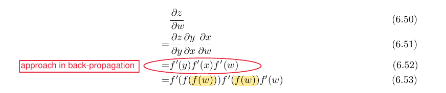 is clearly preferable because of its reduced runtime. However, equation 6.53 is also a valid implementation of the chain rule, and is useful when memory is limited.” (Goodfellow, Bengio)
Softmax
- Softmax loss:
- die inputs $\mathbf{w}_k^\top\mathbf{x}$ und $\mathbf{w}_j^\top\mathbf{x}$ für $j=1,\ldots,K$ kommen vom vorigen FC layer (
.Linearlayer), d.h. die $\mathbf{w}_j$ sind Spalten der FC layer parameter Matrix $\mathbf{W}$ - der Softmax layer selbst hat keine Parameter
- der Softmax layer kann als eine Art activation function gesehen werden, der $\mathbf{Wx}$ transformiert [ähnlich wie RELU]
- die inputs $\mathbf{w}_k^\top\mathbf{x}$ und $\mathbf{w}_j^\top\mathbf{x}$ für $j=1,\ldots,K$ kommen vom vorigen FC layer (
- [source] Softmax is a parameter free activation function like RELU, Tanh or Sigmoid: it doesn’t need to be trained. It only computes the exponential of every logit and then normalize the output vector by the sum of the exponentials.

Implementing Softmax Correctly
- Problem: Exponentials get very big and can have very different magnitudes
- Solution:
- Evaluate $\ln{(\sum_{j=1}^K\exp{(\mathbf{w}_j^\top\mathbf{x})})}$ in the denominator before calculating the fraction
- since $\text{softmax}(\mathbf{a} + \mathbf{b}) = \text{softmax}(\mathbf{a})$ for all $\mathbf{b}\in\mathbb{R}^D$, one can subtract the largest $\mathbf{w}_j$ from the others
- (entspricht $\mathbf{a}=\mathbf{w}_j^\top\mathbf{x}$ und $\mathbf{b}=\mathbf{w}_M^\top\mathbf{x}$ bzw. Kürzen des Bruches mit $\exp{(\mathbf{w}_M^\top\mathbf{x})}$, wobei $\mathbf{w}_M$ das größte weight ist)
- (egal, ob $\mathbf{b}$ von $\mathbf{x}$ abhängt oder nicht!)
- Solution:
MLP in numpy from scratch
- see here
Stochastic Learning vs Batch Learning
[source: LeCun et al. “Efficient BackProp”]
SGD (one at a time)
Pros
- Pros:
- is usually much faster than batch learning
- consider large redundant data set
- example: training set of size 1000 is inadvertently composed of 10 identical copies of a set with 100 samples
- consider large redundant data set
- also often results in better solutions because of the noise in the updates
- because the noise present in the updates can result in the weights jumping into the basin of another, possibly deeper, local minimum. This has been demonstrated in certain simplified cases
- can be used for tracking changes
- useful when the function being modeled is changing over time
- Small batches can offer a regularizing effect (Wilson and Martinez, 2003), perhaps due to the noise they add to the learning process. Generalization error is often best for a batch size of 1.
- is usually much faster than batch learning
Cons
- Cons:
- noise also prevents full convergence to the minimum
- Instead of converging to the exact minimum, the convergence stalls out due to the weight fluctuations:
- size of the fluctuations depend on the degree of noise of the stochastic updates:
- The variance of the fluctuations around the local minimum is proportional to the learning rate $\eta$
- which in turn is inversely proportional to the number of patterns presented $\eta\propto\frac{c}{t}$ [see paper]
- The variance of the fluctuations around the local minimum is proportional to the learning rate $\eta$
- “So in order to reduce the fluctuations we can either”
- “decrease (anneal) the learning rate or”
- start with large $\eta$ and decrease $\eta$ as the training proceeds
- “have an adaptive batch size.”
- start with small mini-batch size $t$ and increase mini-batch size $t$ as the training proceeds - determining an appropriate $t$ is as difficult as determining an appropriate $\eta$ and, therefore, methods (i) and (ii) are equally efficient at reducing these weight fluctuations
- Note: This is only valid in the noise regime at the end of training and not a general rule for training!
- in the beginning of the training for a non-convex, non-quadratic error surface simple rules like this one do not apply, i.e. increasing the mini-batch size may have a different effect than decreasing the learning rate!
- “decrease (anneal) the learning rate or”
- however, this weight fluctuation problem may be “less severe than one thinks because of generalization”
- i.e. “Overtraining may occur long before the noise regime is even reached.”
- size of the fluctuations depend on the degree of noise of the stochastic updates:
- Instead of converging to the exact minimum, the convergence stalls out due to the weight fluctuations:
- noise also prevents full convergence to the minimum
Convergence
- konvergiert nicht immer, im Ggs. zu Batch GD!
- Wikipedia “SGD”:
- The convergence of stochastic gradient descent has been analyzed using the theories of convex minimization and of stochastic approximation.
- Briefly, when the learning rates $\eta$ decrease with an appropriate rate, and subject to relatively mild assumptions, stochastic gradient descent converges almost surely to a global minimum when the objective function is convex or pseudoconvex, and otherwise converges almost surely to a local minimum.
- This is in fact a consequence of the Robbins-Siegmund theorem.
- Wikipedia “SGD”:
Batch GD (entire training set)
- Pros:
- Conditions of convergence are well understood.
- Many acceleration techniques (most 2nd order methods, e.g. conjugate gradient) only operate in batch learning.
- Theoretical analysis of the weight dynamics and convergence rates are simpler
- Cons:
- redundancy can make batch learning much slower than on-line
- often results in worse solutions because of the absence of noise in the updates
- will discover the minimum of whatever basin the weights are initially placed
- changes go undetected and we obtain rather bad results since we are likely to average over several rules
Mini-batch GD
- LeCun “Efficient BackProp”:
- Another method to remove noise [in SGD] is to use “mini-batches”, that is, start with a small batch size and increase the size as training proceeds.
- However, deciding the rate at which to increase the batch size and which inputs to include in the small batches is as difficult as determining the proper learning rate. Effectively the size of the learning rate in stochastic learning corresponds to the respective size of the mini batch.
- Note also that the problem of removing the noise in the data may be less critical than one thinks because of generalization. Overtraining may occur long before the noise regime is even reached.
- Another method to remove noise [in SGD] is to use “mini-batches”, that is, start with a small batch size and increase the size as training proceeds.
- [Jastrzębski, S., Kenton, Z., Arpit, D., Ballas, N., Fischer, A., Bengio, Y., & Storkey, A., (2018, October), “Width of Minima Reached by Stochastic Gradient Descent is Influenced by Learning Rate to Batch Size Ratio”]
- The authors give the mathematical and empirical foundation to the idea that the ratio of learning rate to batch size influences the generalization capacity of DNN. They show that this ratio plays a major role in the width of the minima found by SGD. The higher ratio the wider is minima and better generalization. source
Hyperparameter Tuning and Optimization
Manual Hyperparameter Search
- The primary goal of manual hyperparameter search is to adjust the effective capacity of the model to match the complexity of the task.
Overfitting
- Problem: training error and test error diverge (see below: generalization gap), if we use too many parameters
- Causes:
- large $\mathbf{w}$ magnitudes
- Solution:
- add weight decay/regularization term
- does not reduce the generalization gap, but rather reduces the capacity of the model!
- Dropout (i.e. randomly switching off units during training)
- data augmentation (i.e. artificially enlarge the dataset using label-preserving transformation)
- (validation-based) early stopping
- split training data into training and test set
- train only on training set and evaluate test error once in a while (e.g. after every 5th epoch)
- stop training as soon as error on test set is higher than it was the last time it was checked
- use the weights the NN had in the previous iteration as final weights
- extension: use cross-validation
- complication: multiple local minima
- there are many ad hoc rules to decide when overfitting has truly begun
- reduce number of parameters (if there is no other way)
- use a different model
- use transfer learning
- add weight decay/regularization term
Capacity
Forms of Capacity
- Goodfellow_2016
- representational capacity of a model
- which family of functions the learning algorithm can choose from when varying the parameters
- effective capacity
- the effective capacity may be less than the representational capacity because of additional limitations, e.g.:
- imperfection of the optimization algorithm: in practice, the learning algorithm does not actually find the best function, but merely one that significantly reduces the training error.
- the effective capacity may be less than the representational capacity because of additional limitations, e.g.:
- representational capacity of a model
- Goodfellow_2016
- Effective capacity is constrained by three factors:
- the representational capacity of the model,
- the ability of the learning algorithm to successfully minimize the cost function used to train the model, and
- the degree to which the cost function and training procedure regularize the model.
- A model with more layers and more hidden units per layer has higher representational capacity - it is capable of representing more complicated functions.
- It can not necessarily actually learn all of these functions though, if the training algorithm cannot discover that certain functions do a good job of minimizing the training cost, or if regularization terms such as weight decay forbid some of these functions.
- Effective capacity is constrained by three factors:
Changing a Model’s Capacity
- Goodfellow_2016
- [Representation Capacity:]
- by changing the number of input features it [the model] has,
- and simultaneously adding new parameters associated with those features
- Note:
- In polynomial regression example:
- nur ein input feature (mit polynomial basis function)
- In polynomial regression example:
- by changing the number of input features it [the model] has,
- [Effective Capacity:]
- see forms_capacity
- [Representation Capacity:]
Quantifying a Model’s Capacity (Statistical Learning Theory)
- VC dimension
- The most important results in statistical learning theory show that
- (Vapnik and Chervonenkis, 1971; Vapnik, 1982; Blumer et al., 1989; Vapnik, 1995)
- the discrepancy between training error and generalization error [“generalization gap”] is bounded from above by a quantity that
- grows as the model capacity grows but
- shrinks as the number of training examples increases.
- these bounds provide intellectual justification that machine learning algorithms can work
- however, these bounds are rarely used in practice because:
- bounds are often quite loose
- it is difficult to determine the capacity of deep learning models
- because “effective capacity is limited by the capabilities of the optimization algorithm, and we have little theoretical understanding of the very general non-convex optimization problems involved in deep learning.”
- the discrepancy between training error and generalization error [“generalization gap”] is bounded from above by a quantity that
- (Vapnik and Chervonenkis, 1971; Vapnik, 1982; Blumer et al., 1989; Vapnik, 1995)
Relationship between Capacity and Error
- terminology: test error = generalization error
- Note: Figure 5.3 shows the capacity on the x-axis and not the training epochs!
 source: Goodfellow_2016
 - basically the same plot as in Bishop_2006 “polynomial curve fitting” training and test error $E_{\text{RMS}}$ vs. order of the polynomial $M$ (where $M$ corresponds to capacity here)
Learning Curve Diagnostics
- training error converges to true error for $N\to\infty$, if data points are i.i.d.
- see Learning Curve Diagnostics and Solutions
- original version, but slightly less content: Jason Brownlee “How to use Learning Curves to Diagnose Machine Learning Model Performance”
Learning Rate
- Goodfellow_2016
- controls the effective capacity of the model in a more complicated way than other hyperparameters
- the effective capacity of the model is highest when the learning rate is correct for the optimization problem, not when the learning rate is especially large or especially small
- The learning rate has a U-shaped curve for training error, illustrated in figure 11.1.
- When the learning rate is too large, gradient descent can inadvertently increase rather than decrease the training error.
- In the idealized quadratic case, this occurs if the learning rate is at least twice as large as its optimal value (LeCun et al., 1998a).
- When the learning rate is too small, training is not only slower, but may become permanently stuck with a high training error.
- This effect is poorly understood (it would not happen for a convex loss function).
- When the learning rate is too large, gradient descent can inadvertently increase rather than decrease the training error.
- controls the effective capacity of the model in a more complicated way than other hyperparameters
Adaptive Learning Rate Methods
Methods, if Directions of Sensitivity are NOT axis-aligned (momentum based methods)
- the smoothing effects of momentum based techniques also result in overshooting and correction. (see Alec Radford)
- handle large / dynamic gradients much more poorly than gradient scaling based algorithms and vanilla SGD
Momentum Method
- start with $0.5$
- once the large gradients have disappeared (plot gradient norm) and the weights are stuck in a ravine increase the momentum to $0.9$ or even $0.99$
Nesterov-accelerated gradient
Methods, if Directions of Sensitivity ARE axis-aligned
Separate, Adaptive Learning Rates based methods
- Hinton, Lecture 6.4 — Adaptive learning rates for each connection:
- only deals with axis-aligned effects [Goodfellow: “If we believe that the directions of sensitivity are somewhat axis-aligned, it can make sense to use a separate learning rate for each parameter, and automatically adapt these learning rates throughout the course of learning.” {d.h. die Achsen sind entlang der $w_{ij}$}]
- as opposed to momentum which can deal with these diagonal ellipses [i.e. correlated $\mathbf{w}_{ij}$] and go in that diagonal direction quickly
- only deals with axis-aligned effects [Goodfellow: “If we believe that the directions of sensitivity are somewhat axis-aligned, it can make sense to use a separate learning rate for each parameter, and automatically adapt these learning rates throughout the course of learning.” {d.h. die Achsen sind entlang der $w_{ij}$}]
- Motivation:
- magnitudes of gradients very different for different layers (smaller in early layers)
- therefore, learning rates should be allowed to be different for different layers
- fan-in very different for different layers (the fan-in determines size of “overshoot” effect: the larger the fan-in of a unit the more prone to overshooting the “local minimum for that unit”)
- therefore, learning rates should be allowed to be different for different
unitslayers (assuming the fan-in is the same for all units in a layer) - therefore, weights should be initialized inversely proportional to the fan-in of the units $\Rightarrow$ Glorot initialization
- therefore, learning rates should be allowed to be different for different
- magnitudes of gradients very different for different layers (smaller in early layers)
Robert A. Jacobs’ method (delta-bar-delta algorithm)
- idea: a change of gradient sign indicates that the last update was too big and that the algorithm has jumped over a local minimum
- designed for full batch learning
- use large minibatch
- ensures that changes of sign are not due to sampling error of a minibatch, but due to really going to the other side of the ravine
- use large minibatch
- global learning rate multiplied by a local gain per weight
- ensures that big gains decay rapidly when oscillations across a ravine start
- Note: unlike Rprop this method uses
- the gradient magnitude
- an additive increase (in Rprop: multiplicative increase)
- Robert A. Jacobs, 1988
- delta-bar-delta algorithm
Rprop
- only for full batch learning
- why: Rprop violates the fundamental property of SGD “averaging over minibatches” (i.e. over sufficiently many minibatches the SGD gradient will approximate the full batch gradient)
- Rprop gradients $\frac{\textbf{grad}}{\Vert grad\Vert}$ always have magnitude 1, so that “magnitudinal averaging” is not possible over minibatches (although “directional averaging” would be possible, but, since the gradients always have magnitude 1, this “directional averaging” does not work, too)
- make it work for minibatches, enforce “averaging over minibatches” $\Rightarrow$ RMSprop
- why: Rprop violates the fundamental property of SGD “averaging over minibatches” (i.e. over sufficiently many minibatches the SGD gradient will approximate the full batch gradient)
- local learning rate per weight (unlike RMSprop), but global gain $\eta^+$ or $\eta^-$ respectively
- one initial learning rate $\gamma_{ij}^{(0)}$ per weight $w_{ij}$ which will be updated in each iteration by a global gain $\eta^+$ or $\eta^-$ respectively
- Hinton, Lecture 6.5 — Rmsprop: normalize the gradient:
- for issues like escaping from plateaus with very small gradients this is a great technique
- because even with tiny gradients we will take quite big steps
- we could not achieve that just by turning up the learning rate because then the steps we took for weights that had big gradients would be much too big
- combines the idea of just using the sign of the gradient with the idea of making the step size depend on which weight it is
- so to decide how much to change a weight
- you don’t look at the magnitude of the gradient $\frac{\partial E}{\partial w_{ij}}$,
- we just look at the sign of the gradient $\frac{\partial E}{\partial w_{ij}}$,
- but you do look at the step size $\eta_{ij}$ that you have decided on for that weight and that step size adapts over time, again, without looking at the magnitude of the gradient
- increase step size multiplicatively (if last 2 gradient signs agree)
- as opposed to Robert Jacobs’ “Adpative Learning Rate” method which increases additively
- decrease step size multiplicatively (if last 2 gradient signs disagree)
- increase step size multiplicatively (if last 2 gradient signs agree)
- so to decide how much to change a weight
- for issues like escaping from plateaus with very small gradients this is a great technique
Gradient Scaling based methods
AdaGrad
- Goodfellow_2016:
- “The AdaGrad algorithm, shown in algorithm 8.4,
- individually adapts the learning rates of all model parameters by scaling them inversely proportional to the square root of the sum of all [im Ggs. zu RMSprop] of their historical squared values (Duchi et al., 2011).
- [Effekt wie bei Momentum, nur axis-aligned error surface contours]
- The parameters with the largest partial derivative of the loss [largest gradients] have a correspondingly rapid decrease in their learning rate, while parameters with small partial derivatives [small gradients] have a relatively small decrease in their learning rate.
- The net effect is greater progress in the more gently sloped directions of parameter space [wie bei Momentum].
- The parameters with the largest partial derivative of the loss [largest gradients] have a correspondingly rapid decrease in their learning rate, while parameters with small partial derivatives [small gradients] have a relatively small decrease in their learning rate.
- empirically it has been found that - for training deep neural network models - the accumulation of squared gradients from the beginning of training can result in a premature and excessive decrease in the effective learning rate.
- AdaGrad performs well for some but not all deep learning models.
- “The AdaGrad algorithm, shown in algorithm 8.4,
RMSprop
- Hinton 2012
- global learning rate
- eigentlich eine Verbesserung von AdaGrad:
- Zaheer, Shaziya, “A Study of the Optimization Algorithms in Deep Learning”:
- RMSProp changes
theadagrad in a way how the gradient is accumulated.- Gradients are accumulated into an exponentially weighted average.
- RMSProp discards the history and maintains only recent gradient information.
- RMSProp changes
- Zaheer, Shaziya, “A Study of the Optimization Algorithms in Deep Learning”:
- Goodfellow_2016
- RMSProp uses an exponentially decaying average to discard history from the extreme past so that it can converge rapidly after finding a convex bowl, as if it were an instance of the AdaGrad algorithm initialized within that bowl.
- Compared to AdaGrad, the use of the moving average introduces a new hyperparameter, $\rho$, that controls the length scale of the moving average.
- Andrew Ng, Oscillation sketch:
- Richtung für jede Dimension/Achse $w_{ij}$ wird über sign of gradient gegeben.
- Betrag für jede Dimension wird über EMA gegeben (global learning rate kann sich ja nicht ändern!), weshalb oszillierende Dimensionen gedämpft werden und nicht oszillierende Dimensionen gleich bleiben bzw. sich etwas verzögert an Änderungen anpassen.
- Hinton:
- Motivation: “Rprop for mini-batch learning”
- Rprop is equivalent to using the gradient, but also dividing by the magnitude of the gradient
- problem: we divide by a different magnitude for each mini-batch!
- I.e. the core idea of SGD of stochastic “averaging of weight updates over mini-batches” is violated
- in other words, the weight update noise is not the same as in standard mini-batch SGD !
- solution: force the number we divide by to be pretty much the same for nearby mini-batches
- problem: we divide by a different magnitude for each mini-batch!
- Rprop is equivalent to using the gradient, but also dividing by the magnitude of the gradient
- combines
- the robustness of Rprop (which allows to combine gradients in the right way)
- efficiency of mini-batches
- averaging of gradients over mini-batches
- Hinton:
- notice, that we are not adapting the learning rate separately for each connection here!
- This is a simpler method, where we simply, for each connection, keep a running average of the root mean square gradient and divide by that.
- Extensions:
- can be combined with momentum, but does not help as much as momentum normally does
- that needs more investigation
- can be combined with adaptive learning rates for each connection
- Hinton: “That needs more investigation. I just do not know how helpful that will be.”
- can be combined with momentum, but does not help as much as momentum normally does
- Motivation: “Rprop for mini-batch learning”

RMSProp with Nesterov Momentum
Adam
- Kingma, Ba 2014
- Goodfellow_2016
- The name “Adam” derives from the phrase “adaptive moments.”
- In the context of the earlier algorithms, it is perhaps best seen as a variant on the combination of RMSProp and momentum [s.o] with a few important distinctions.
Learning rate schedules
- can be used instead of using “adaptive learning rate methods” (see above)
- source:
- A learning rate schedule changes the learning rate during learning and is most often changed between epochs/iterations.
- This is mainly [in most implementations] done with two parameters:
- decay
- momentum
- There are many different learning rate schedules but the most common are time-based, step-based and exponential.
Saddle Points and Local Minima
Hessian (2nd derivative test)
- When the Hessian is positive definite (all its eigenvalues are positive), the point is a local minimum.
- when the Hessian is negative definite (all its eigenvalues are negative), the point is a local maximum.
- In multiple dimensions, it is actually possible to find positive evidence of saddle points in some cases.
- When at least one eigenvalue is positive and at least one eigenvalue is negative, we know that $x$ is a local maximum on one cross section of $f$ but a local minimum on another cross section.
- The test is inconclusive whenever all of the non-zero eigenvalues have the same sign, but at least one eigenvalue is zero.
The Condition Number of the Hessian
- tool, um “long canyon” Probleme (i.e. “krümmungsbasierte” Konvergenzprobleme) zu messen

- Goodfellow_2016:
- “In multiple dimensions, there is a different second derivative for each direction at a single point. The condition number of the Hessian at this point measures how much the second derivatives differ from each other.”
- "When the Hessian has a poor condition number, **gradient descent performs poorly**."
- “This is because in one direction, the derivative increases rapidly, while in another direction, it increases slowly. Gradient descent is unaware of this change in the derivative” [“unaware”, weil “change in the derivative” mit Hessian gemessen wird und GD Hessian nicht benutzt]
- information about the change in the function is contained in 1st derivative
- information about the change in the derivative is contained in the 2nd derivative!
- “so it does not know that it needs to explore preferentially in the direction where the derivative remains negative for longer.”
- “This is because in one direction, the derivative increases rapidly, while in another direction, it increases slowly. Gradient descent is unaware of this change in the derivative” [“unaware”, weil “change in the derivative” mit Hessian gemessen wird und GD Hessian nicht benutzt]
- "When the Hessian has a poor condition number, **gradient descent performs poorly**."
- “In multiple dimensions, there is a different second derivative for each direction at a single point. The condition number of the Hessian at this point measures how much the second derivatives differ from each other.”
The proliferation of saddle points in higher dimensions
- Goodfellow_2016:
- At a saddle point, the Hessian matrix [important tool for analyzing critical points, e.g. determine Eigenvalues to check, if it is a saddle point, a local minimum or a maximum] has both positive and negative eigenvalues.
- Points lying along eigenvectors associated with positive eigenvalues have greater cost than the saddle point, while points lying along negative eigenvalues have lower value.
- Bengio, summer school lecture
- wrong idea: non-convex error surface $\Rightarrow$ many local minima $\Rightarrow$ we don’t get any guarantees to find the optimal solution and furthermore, we might be stuck in very poor solutions
- one of the reasons why researchers lost interest in NNs
- there is theoretical and empirical evidence that this issue of non-convexity is not an issue at all
- Pascanu, Dauphin, Ganguli, Bengio
- Dauphin, Pascanu, Gulcehre, Cho, Ganguli, Bengio
- Choromanska, Henaff, Mathieu, Ben Arous & LeCun
- these papers describe saddle points in high dimensions:
- for a local minimum all the directions starting from the critical point (i.e. derivative equal to zero) must go up (and for a local maximum v.v.)
- the more dimensions you have the more “unlikely” (if you construct a function with some randomness and you choose independently whether a direction starting from the critical point goes up or down) it gets that all the directions go up at a critical point
- this gets exponentially more unlikely with each additional dimension!
- except, if you are at the bottom of your high-dimensional landscape, i.e. near the global minimum
- because if you have a minimum near the global minimum you cannot go further down, so all the directions have to go up
- this means, you have local minima [for high-dimensional functions], but they are very close to the global minimum in terms of their objective function
- because if you have a minimum near the global minimum you cannot go further down, so all the directions have to go up
- Note in talk: “Of course, you could always construct a high-dimensional function, where there is a local minimum which is not close to the global minimum. You could just place a local minimum by hand at some higher point of the error surface. I just argue that local minima are very likely not the problem, when training gets stuck.”
- plot: training error and norm of the gradients:
- you see the error go down and it plateaus and then, if you are lucky, something happens and then it goes down again and it plateaus again and then we might think this is the best we can get, but the gradients do not approach zero, what’s going on?
- this looks like we are approaching a saddle point
- my intuition is that this such a high-dimensional space that there is only a few dimensions where it is going down and somehow simple Gradient Descent is not finding them (maybe because of curvature problems [Goodfellow_2016, Fig. 4.5] or other things)
- What I’m saying is, yes, it is worthwhile to continue exploring other optimization algorithms beyond simple GD, but we need to take into account the fact that maybe what we are fighting is not local minima, it might be something else. It might be something classical like differences of curvature or something more subtle.
- as you go further down it spends more and more time on these plateaus (and it gets harder and harder to decide whether we are still on a saddle point), presumably because there are less directions going down [i.e. we are close to the global minimum]
- cite: Goodfellow_2016:
- experts now suspect that, for sufficiently large neural networks, most local minima have a low cost function value, and that it is not important to find a true global minimum rather than to find a point in parameter space that has low but not minimal cost
- Many practitioners attribute nearly all difficulty with neural network optimization to local minima.
- We encourage practitioners to carefully test for specific problems.
- A test that can rule out local minima as the problem is to plot the norm of the gradient over time. If the norm of the gradient does not shrink to insignificant size [same problem as discussed here], the problem is neither local minima nor any other kind of critical point. [then it’s either a saddle point or something more subtle]
- This kind of negative test can rule out local minima.
- [also einfach beim training die Gradient Norm mitplotten und nur wenn diese Norm plötzlich 0 wird ist es ein local Minimum, sonst nicht!]
- [those practitioners are wrong because] In high dimensional spaces, it can be very difficult to positively establish that local minima are the problem. Many structures other than local minima also have small gradients.
- We encourage practitioners to carefully test for specific problems.
- you see the error go down and it plateaus and then, if you are lucky, something happens and then it goes down again and it plateaus again and then we might think this is the best we can get, but the gradients do not approach zero, what’s going on?
- Note in talk: stopping criterion? You should be ready to wait. People discarded NNs in part because they were not ready to wait long enough (when I was a PhD student, we were ready to wait weeks, people are getting lazy these days ;))
- these papers describe saddle points in high dimensions:
- wrong idea: non-convex error surface $\Rightarrow$ many local minima $\Rightarrow$ we don’t get any guarantees to find the optimal solution and furthermore, we might be stuck in very poor solutions
- source
- The team of Yoshua Bengio have experimentally found that when optimising the parameters of high-dimensional neural nets, there effectively are no local minima. Instead, there are saddle points which are local minima in some dimensions but not all. This means that training can slow down quite a lot in these points, until the network figures out how to escape, but as long as we’re willing to wait long enough then it will find a way.
- Given one specific dimension, there is some small probability $p$ with which a point is a local minimum, but not a global minimum, in that dimension. Now, the probability of a point in a $1000$-dimensional space being an incorrect local minimum in all of these would be $p^{1000}$, which is just astronomically small. However, the probability of it being a local minimum in some of these dimensions is actually quite high. And when we get these minima in many dimensions at once, then training can appear to be stuck until it finds the right direction.
- In addition, this probability $p$ will increase as the loss function gets closer to the global minimum. This means that if we do ever end up at a genuine local minimum, then for all intents and purposes it will be close enough to the global minimum that it will not matter.
- Goodfellow_2016
- For many high-dimensional non-convex functions, local minima (and maxima) are in fact rare compared to another kind of point with zero gradient: a saddle point.
- Some points around a saddle point have greater cost than the saddle point, while others have a lower cost.
- At a saddle point, the Hessian matrix has both positive and negative eigenvalues.
- Points lying along eigenvectors associated with positive eigenvalues have greater cost than the saddle point, while points lying along negative eigenvalues have lower value.
- We can think of a saddle point as being a local minimum along one cross-section [sozusagen als würde man mit einer Ebene senkrecht durch den Graph schneiden] of the cost function and a local maximum along another cross-section. See figure 4.5 for an illustration.
Shuffling/Ordering/Emphasizing Schemes
Shuffling
- irrelevant for full batch learning
- Example: Within the training set, the images are ordered in such a way that all the dog images come first and all the cat images come after. The classes are balanced.
- Effect: The optimization is much harder with mini-batch gradient descent because the loss function moves by a lot when going from the one type of image to another.
- Solution: Shuffle before training
Ordering
- Müller, Montavon:
- Networks learn the fastest from the most unexpected sample. Therefore, it is advisable to **choose a sample at each iteration that is the most unfamiliar to the system**.
- Note, this applies only to stochastic learning since the order of input presentation is irrelevant for batch.
- [Method 1 for “choose a sample at each iteration that is the most unfamiliar to the system”:] Of course, there is no simple way to know which inputs are information rich,
- however, a very simple trick that crudely implements this idea is to simply choose successive examples that are from different classes since training examples belonging to the same class will most likely contain similar information.
- Networks learn the fastest from the most unexpected sample. Therefore, it is advisable to **choose a sample at each iteration that is the most unfamiliar to the system**.
Emphasizing Schemes
- Müller, Montavon:
- [Method 2 for “choose a sample at each iteration that is the most unfamiliar to the system”:] Another heuristic for judging how much new information a training example contains is to examine the error between the network output and the target value when this input is presented.
- A large error indicates that this input has not been learned by the network and so contains a lot of new information.
- Therefore, it makes sense to present this input more frequently.
- Of course, by “large” we mean relative to all of the other training examples.
- As the network trains, these relative errors will change and so should the frequency of presentation for a particular input pattern.
- A method that modifies the probability of appearance of each pattern is called an **emphasizing scheme**.
- However, one must be careful when perturbing the normal frequencies of input examples because this changes the relative importance that the network places on different examples. This may or may not be desirable.
- For example, this technique applied to data containing outliers can be disastrous because outliers can produce large errors yet should not be presented frequently.
- On the other hand, this technique can be particularly beneficial for boosting the performance for infrequently occurring inputs, e.g. /z/ in phoneme recognition.
- [Method 2 for “choose a sample at each iteration that is the most unfamiliar to the system”:] Another heuristic for judging how much new information a training example contains is to examine the error between the network output and the target value when this input is presented.
Transforming the inputs (shift, scale, decorrelate)
- Note: many possible methods for image data:
- normalization, centering, standardization
- also many possible orders in which these steps are done
- normalization, centering, standardization
- Note: source
- Normalizing the input impacts the landscape of the loss function.
- The normalizing mean and variance computed on the training set, and used to train the model, should be used to normalize test data.
- Hinton, Lecture 6.2 — A bag of tricks for mini batch gradient descent:
- red line corresponds to the bottom of the “trough” defined by the training point $x_1=(101,99)$, the corresponding output of the simple 2 unit NN shown below is $0$
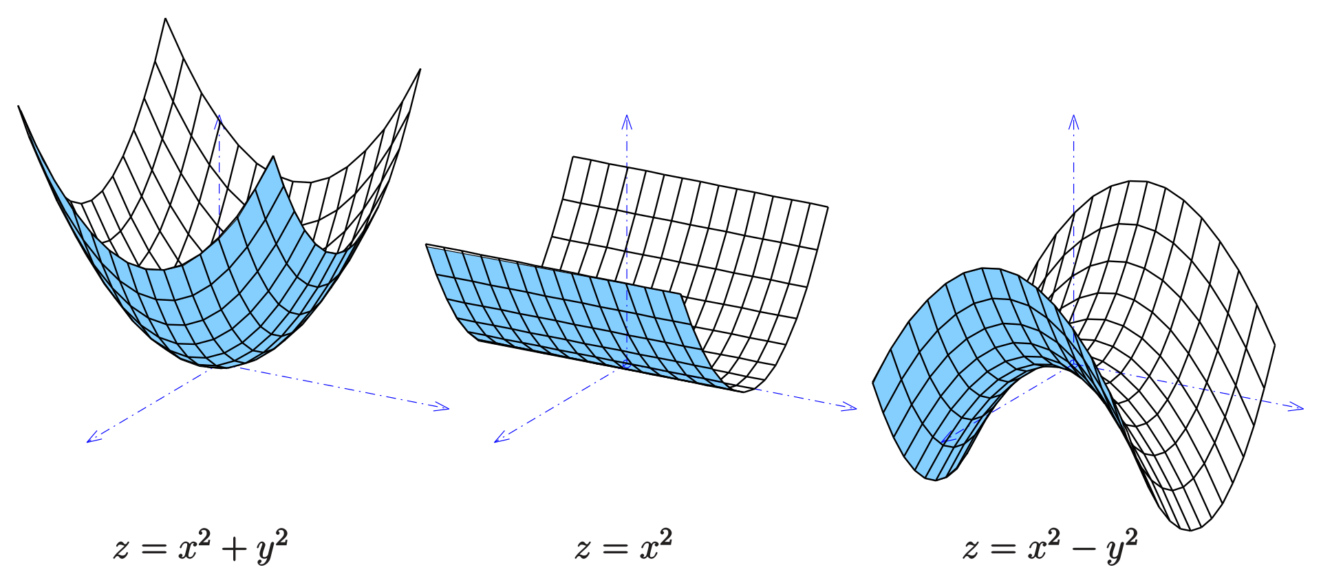
- “trough” in 2-D: “parabolic cylinder”, see below: graph in the middle: $z=x^2$
- superposition of two parabolic cylinders results in an elliptic paraboloid, see below: left graph: $z=x^2+y^2$
- this is why $x_1$ and $x_2$ together form an elliptic paraboloid error surface
- superposition of two parabolic cylinders results in an elliptic paraboloid, see below: left graph: $z=x^2+y^2$
- “trough” in 2-D: “parabolic cylinder”, see below: graph in the middle: $z=x^2$
- green line corresponds to the bottom of the “trough” defined by the training point $x_2=(101,101)$, the corresponding output of the simple 2 unit NN shown below is $2$
- the black ellipse corresponds to the contours of the error surface (which in 2-D has the shape of an elliptic paraboloid)
- this ellipse has a very elongated shape because $x_1$ and $x_2$ are both positive and do not have average zero
- steepest descent methods have difficulties with such “troughs”
- slows down learning
- shifting the inputs, so that the average over the whole training set is close to zero makes the error surface contours more circular (see below)
- speeds learning with steepest descent
- this ellipse has a very elongated shape because $x_1$ and $x_2$ are both positive and do not have average zero
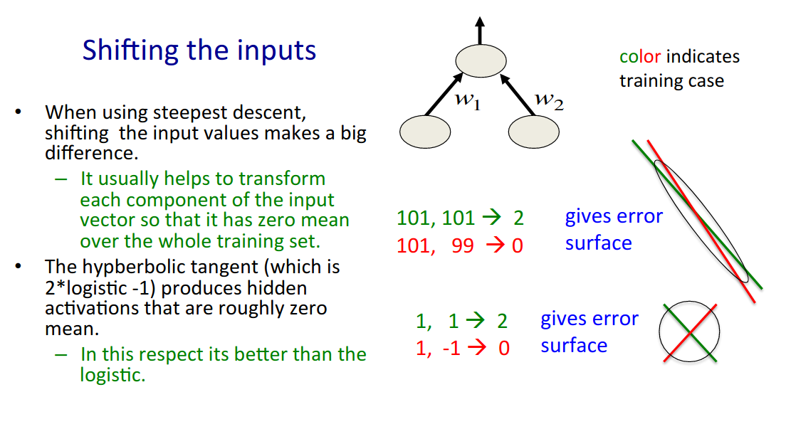
- red line corresponds to the bottom of the “trough” defined by the training point $x_1=(101,99)$, the corresponding output of the simple 2 unit NN shown below is $0$
- LeCun “Efficient BackProp”:
- “The average of each input variable over the training set should be close to zero.”
- When all of the components of an input vector are positive, all of the updates of weights that feed into a node will be the same sign (i.e. $\text{sign}(\delta)$).
- biases the updates in a particular direction
- As a result, these weights can only all decrease or all increase together for a given input pattern.
- Thus, if a weight vector must change direction it can only do so by zigzagging which is inefficient and thus very slow.

- Thus, if a weight vector must change direction it can only do so by zigzagging which is inefficient and thus very slow.
- In the above example, the inputs were all positive. However, in general, any shift of the average input away from zero will bias the updates in a particular direction and thus slow down learning.
- Therefore, it is good to shift the inputs so that the average over the training set is close to zero.
- This heuristic should be applied at all layers which means that we want the average of the outputs of a node to be close to zero because these outputs are the inputs to the next layer [19], chapter 10.
- This problem can be addressed by coordinating how the inputs are transformed with the choice of sigmoidal activation function.
- This heuristic should be applied at all layers which means that we want the average of the outputs of a node to be close to zero because these outputs are the inputs to the next layer [19], chapter 10.
- When all of the components of an input vector are positive, all of the updates of weights that feed into a node will be the same sign (i.e. $\text{sign}(\delta)$).
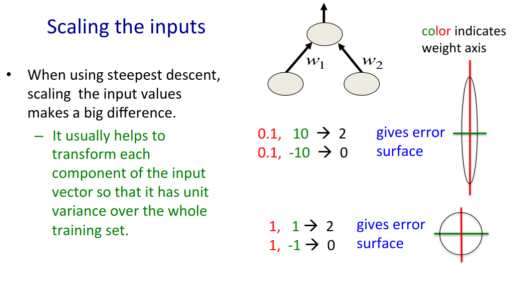
- “Scale input variables so that their covariances are about the same.”
- helps to balance out the rate at which the weights connected to the input nodes learn.
- The value of the covariance should be matched with that of the sigmoid used.
- The exception to scaling all covariances to the same value occurs
- when it is known that some inputs are of less significance than others.
- In such a case, it can be beneficial to scale the less significant inputs down so that they are “less visible” to the learning process
- when it is known that some inputs are of less significance than others.
- “Input variables should be uncorrelated if possible.”
- If inputs are uncorrelated then it is possible to solve for the value of $w_1$ that minimizes the error without any concern for $w_2$, and vice versa.
- In other words, the two variables are independent (the system of equations is diagonal).
- With correlated inputs, one must solve for both simultaneously which is a much harder problem.
- Principal component analysis (also known as the Karhunen-Loeve expansion) can be used to remove linear correlations in inputs [10].
- Inputs that are linearly dependent (the extreme case of correlation) may also produce degeneracies which may slow learning.
- Consider the case where one input is always twice the other input ($z_2 = 2z_1$).
- We are trying to solve in 2-D what is effectively only a 1-D problem.
- Ideally we want to remove one of the inputs which will decrease the size of the network.
- Summary:
- Consider the case where one input is always twice the other input ($z_2 = 2z_1$).
- (1) shift inputs so the mean is zero,
- (2) decorrelate inputs, and
- (3) equalize covariances.
- If inputs are uncorrelated then it is possible to solve for the value of $w_1$ that minimizes the error without any concern for $w_2$, and vice versa.
- “The average of each input variable over the training set should be close to zero.”
Sigmoids
- LeCun, “Efficient BackProp”:
- Symmetric sigmoids such as hyperbolic tangent [$\tanh$] often converge faster than the standard logistic function.
- A recommended sigmoid is: $f(x) = 1.7159\tanh\frac{2}{3}x$. Since the $\tanh$ function is sometimes computationally expensive, an approximation of it by a ratio of polynomials can be used instead.
- The constants in the recommended sigmoid given above have been chosen so that, when used with transformed inputs (see previous discussion), the variance of the outputs will also be close to 1
- because the effective gain of the sigmoid is roughly 1 over its useful range.
- Properties:
- (a) $f(±1) = ±1$,
- [why good? später im Text] set the target values [d.h. 1 und -1] to be within the range of the sigmoid, rather than at the asymptotic values [and at the same time] ensure that the node is not restricted to only the linear part
- (b) the second derivative is a maximum at $x = 1$ [siehe “1.4.5 Choosing Target Values”], and
- [why good? später im Text] Setting the target values to the point of the maximum second derivative on the sigmoid is the best way to take advantage of the nonlinearity without saturating the sigmoid.
- (c) the effective gain is close to $1$.
- [why good?] if the variance of the inputs is 1, then the variance of the outputs will also be close to 1
- (a) $f(±1) = ±1$,
- The constants in the recommended sigmoid given above have been chosen so that, when used with transformed inputs (see previous discussion), the variance of the outputs will also be close to 1
- Sometimes it is helpful to add a small linear term, e.g. $f(x) = \tanh(x) + ax$ so as to avoid flat spots.
- One of the potential problems with using symmetric sigmoids is that the error surface can be very flat near the origin.
- For this reason it is good to avoid initializing with very small weights.
- Because of the saturation of the sigmoids, the error surface is also flat far from the origin.
- Adding a small linear term to the sigmoid can sometimes help avoid the flat regions (see chapter 9).
- One of the potential problems with using symmetric sigmoids is that the error surface can be very flat near the origin.
- Sigmoids that are symmetric about the origin are preferred for the same reason that inputs should be normalized, namely, because they are more likely to produce outputs (which are inputs to the next layer) that are on average close to zero.
Biases Initialization
- Goodfellow_2016
- Typically, we set the biases for each unit to heuristically chosen constants, and initialize only the weights randomly.
- The approach for setting the biases must be coordinated with the approach for settings the weights. Setting the biases to zero is compatible with most weight initialization schemes. There are a few situations where we may set some biases to non-zero values … (see Goodfellow_2016)
- perform a grid search [Le, Hinton 2015]
Weight initialization
Why does it matter?
- Goodfellow_2016
- The initial point can determine whether the algorithm converges at all, with some initial points being so unstable that the algorithm encounters numerical difficulties and fails altogether.
- When learning does converge, the initial point can determine
- how quickly learning converges and
- whether it converges to a point with high or low cost.
- Also, points of comparable cost can have wildly varying generalization error, and the initial point can affect the generalization as well
Open Questions
- Modern initialization strategies are simple and heuristic [i.e. strategies work, but we do not know why].
- Designing improved initialization strategies is a difficult task because neural network optimization is not yet well understood.
- Most initialization strategies are based on achieving some nice properties when the network is initialized.
- However, we do not have a good understanding of which of these properties are preserved under which circumstances after learning begins to proceed.
- A further difficulty is that some initial points may be beneficial from the viewpoint of optimization but detrimental from the viewpoint of generalization.
- Our understanding of how the initial point affects generalization is especially primitive, offering little to no guidance for how to select the initial point.
Symmetry breaking Problem
- source
- for logistic regression we can initialize the weights with zeros, but for NNs this does not work
- in logistic regression:
- derivative of the binary cross entropy loss with respect to a single dimension in the weight vector $w_i$ is a function of $x_i$, which is in general different than $x_j$ when $i\neq j$
- d.h. weight update der Komponente $w_i$ i.e. $-\eta \frac{\partial E}{\partial w_i}$ wird sich i. Allg. vom weight update der anderen Komponenten $-\eta \frac{\partial E}{\partial w_j}$ mit $i\neq j$ unterscheiden
- aka weights werden asymmetrisch geupdatet
- daher ist 0 initialization kein Problem
- d.h. weight update der Komponente $w_i$ i.e. $-\eta \frac{\partial E}{\partial w_i}$ wird sich i. Allg. vom weight update der anderen Komponenten $-\eta \frac{\partial E}{\partial w_j}$ mit $i\neq j$ unterscheiden
- derivative of the binary cross entropy loss with respect to a single dimension in the weight vector $w_i$ is a function of $x_i$, which is in general different than $x_j$ when $i\neq j$
- in logistic regression:
- Problem: consider 2 layer NN below:
- if $W_1$ and $W_2$ are initialized with constants or with zeros, both hidden units will calculate the same function (i.e. they are symmetric) during forward and backward pass
- i.e. there is no reason to have more than one hidden unit here
- also applies to more than 2 hidden units
- proof by induction:
- first iteration: both hidden units start off by computing the same function
- next iteration: still compute the same function
- by induction: they will always compute the same function during training
- if $W_1$ and $W_2$ are initialized with constants or with zeros, both hidden units will calculate the same function (i.e. they are symmetric) during forward and backward pass
- Solution: break this symmetry by using randomly initialized weights
- too large initialization $\Rightarrow$ sigmoid/tanh will saturate $\Rightarrow$ slows down learning
- Thus initialize with small Gaussian numbers, here $0.01$
- $b$ does not have this “Symmetry breaking problem”, hence, it can be initialized with $0$

- Goodfellow_2016
- Perhaps the only property known with complete certainty is that the initial parameters need to “break symmetry” between different units.
- If two hidden units with the same activation function are connected to the same inputs, then these units must have different initial parameters.
- If they have the same initial parameters, then a deterministic learning algorithm applied to a deterministic cost and model will constantly update both of these units in the same way.
- Even if the model or training algorithm is capable of using stochasticity [as opposed to deterministic updates] to compute different updates for different units (for example, if one trains with dropout), it is usually best to initialize each unit to compute a different function from all of the other units.
- This may help to make sure that no input patterns are lost in the null space of forward propagation and no gradient patterns are lost in the null space of back-propagation.
- Perhaps the only property known with complete certainty is that the initial parameters need to “break symmetry” between different units.
Random Initialization
- Goodfellow_2016
- The goal of having each unit compute a different function motivates random initialization of the parameters.
- We could explicitly search for a large set of basis functions that are all mutually different from each other, but this often incurs a noticeable computational cost.
- For example, if we have at most as many outputs as inputs, we could use Gram-Schmidt orthogonalization on an initial weight matrix, and be guaranteed that each unit computes a very different function from each other unit.
- Random initialization from a high-entropy distribution over a high-dimensional space is computationally cheaper and unlikely to assign any units to compute the same function as each other.
- We could explicitly search for a large set of basis functions that are all mutually different from each other, but this often incurs a noticeable computational cost.
- The goal of having each unit compute a different function motivates random initialization of the parameters.
Biases and other Parameters
- Goodfellow_2016
- Typically, we set the biases for each unit to heuristically chosen constants, and initialize only the weights randomly.
- Extra parameters, for example, parameters encoding the conditional variance of a prediction, are usually set to heuristically chosen constants much like the biases are.
Gaussian or Uniform
- Goodfellow_2016
- We almost always initialize all the weights in the model to values drawn randomly from a Gaussian or uniform distribution.
- The choice of Gaussian or uniform distribution does not seem to matter very much, but has not been exhaustively studied.
- We almost always initialize all the weights in the model to values drawn randomly from a Gaussian or uniform distribution.
Scale
- Goodfellow_2016
- The scale of the initial distribution, however, does have a large effect on both the outcome of the optimization procedure and on the ability of the network to generalize.
- Larger initial weights will yield a stronger symmetry breaking effect, helping to avoid redundant units. They also help to avoid losing signal during forward or back-propagation through the linear component of each layer - larger values in the matrix result in larger outputs of matrix multiplication.
- Initial weights that are too large may, however, result in exploding values during forward propagation or back-propagation.
- In recurrent networks, large weights can also result in chaos (such extreme sensitivity to small perturbations of the input that the behavior of the deterministic forward propagation procedure appears random).
- To some extent, the exploding gradient problem can be mitigated by gradient clipping (thresholding the values of the gradients before performing a gradient descent step).
- Large weights may also result in extreme values that cause the activation function to saturate, causing complete loss of gradient through saturated units.
- In recurrent networks, large weights can also result in chaos (such extreme sensitivity to small perturbations of the input that the behavior of the deterministic forward propagation procedure appears random).
- Initial weights that are too large may, however, result in exploding values during forward propagation or back-propagation.
- These competing factors determine the ideal initial scale of the weights.
- Larger initial weights will yield a stronger symmetry breaking effect, helping to avoid redundant units. They also help to avoid losing signal during forward or back-propagation through the linear component of each layer - larger values in the matrix result in larger outputs of matrix multiplication.
- The scale of the initial distribution, however, does have a large effect on both the outcome of the optimization procedure and on the ability of the network to generalize.
Optimization vs Regularization Perspective
- Goodfellow_2016
- The perspectives of regularization and optimization can give very different insights into how we should initialize a network.
- The optimization perspective suggests that the weights should be large enough to propagate information successfully,
- but some regularization concerns encourage making them smaller.
- The perspectives of regularization and optimization can give very different insights into how we should initialize a network.
Implicit Prior of SGD
- Goodfellow_2016
- The use of an optimization algorithm such as stochastic gradient descent […] expresses a prior that the final parameters should be close to the initial parameters.
Vanishing Gradients Problem
Difference: Sigmoidals vs ReLU
- sigmoidal activation functions have the “vanishing gradients” problem
ReLU does not have a “vanishing gradients” problem!Wrong, ReLU does have the “vanishing gradients” problem! Use He initialization to avoid this problem.Nevertheless, this Xavier initialization (after Glorot’s first name) is a neat trick that works well in practice. However, along came rectified linear units (ReLU), a non-linearity that is scale-invariant around 0 and does not saturate at large input values. This seemingly solved both of the problems the sigmoid function had; or were they just alleviated? I am unsure of how widely used Xavier initialization is, but if it is not, perhaps it is because ReLU seemingly eliminated this problem. http://deepdish.io/
Deepdish explanation
- http://deepdish.io/ What happens for sigmoidal activations?:
- First, let’s go back to the time of sigmoidal activation functions and initialization of parameters using i.i.d. Gaussian or uniform distributions with fairly arbitrarily set variances.
- Building deep networks was difficult because of exploding or vanishing activations and gradients.
- Let’s take activations first:
- If all your parameters are too small,
- the variance of your activations will drop in each layer.
- This is a problem if your activation function is sigmoidal, since it is approximately linear close to 0.
- That is, you gradually lose your non-linearity, which means there is no benefit to having multiple layers.
- If, on the other hand, your activations become larger and larger,
- then your activations will saturate and become meaningless, with gradients approaching 0.
- If all your parameters are too small,
- First, let’s go back to the time of sigmoidal activation functions and initialization of parameters using i.i.d. Gaussian or uniform distributions with fairly arbitrarily set variances.
Code experiment
- vanishing gradients problem: code example (download this directory and view the html file locally, else it does not work)
Leibe
- Leibe:
- Main problem is getting the gradients back to the early layers
- because if the gradients do not come through to the early layers, the early layers will compute random suboptimal features (“garbage”)
- furthermore, since the gradients do not get backpropagated to the early layers those suboptimal features will not get updated and so the training accuracy gets stuck
- for RNNs:
- they severely restrict the dependencies the RNN can learn
- problem gets more severe the deeper the network is
- can be very hard to diagnose that vanishing gradients occur
- you just see that learning gets stuck
- Main problem is getting the gradients back to the early layers
Solutions
- Solutions:
- use LeCun tanh with Glorot/He initialization
- use ReLU with He initialization
- for RNNs:
- more complex hidden units (e.g. LSTM, GRU)
- initialize $\mathbf{W}_{hh}$ with identity matrix and use ReLU
- Le, Hinton 2015:
- The identity initialization has the very desirable property that when the error derivatives for the hidden units are backpropagated through time they remain constant provided no extra error-derivatives are added. This is the same behavior as LSTMs when their forget gates are set so that there is no decay and it makes it easy to learn very long-range temporal dependencies.
- Le, Hinton 2015:
RNNs
- Goodfellow_2016:
- for RNNs: gradients through such a [RNN] graph are also scaled according to $\text{diag}(\vec{\lambda})^t$
- Vanishing gradients make it difficult to know which direction the parameters should move to improve the cost function, while exploding gradients can make learning unstable.
- effect: long-range dependencies are not learned by the RNN
- i.e. words from timesteps far away are not taken into consideration when predicting the next word
Xavier Glorot Initialization
- for tanh nonlinearities
- because the derivation assumes linearity around 0
- Glorot, Bengio paper
- Xavier Glorot is the author’s full name
Kaiming He Initialization
- for ReLU nonlinearities
Dependence on NN depth
- lec 17 (from He et al paper):
- The deeper the NNs are the more the right initialization method matters
- e.g.
- 22-layer ReLU NN will converge with Xavier initialization, although this initialization method is wrong for ReLU nonlinearities
- albeit convergence will be slower than with He initialization
- however, a 30-layer ReLU NN with Xavier initialization will not converge and gets stuck, whereas with He initialization it does converge!
- 22-layer ReLU NN will converge with Xavier initialization, although this initialization method is wrong for ReLU nonlinearities
- e.g.
- The deeper the NNs are the more the right initialization method matters
Dying ReLU problem
- causes:
- too high learning rate
- too large negative bias
- solutions:
- use a lower learning rate
- use a variation of ReLU, e.g.
- Leaky ReLU: $\max{\beta a, a}$
- pro: avoids stuck-at-zero units
- pro: weaker offset bias
- con: does not have the non-informative deactivation states property (cf. below) like ReLU, i.e. inactive Leaky ReLU units carry information because the gradient is not zero for negative inputs!
- PReLU: same as Leaky ReLU, but $\beta$ is a learnable parameter
- ELU: $e^a-1$ for $a \leq 0$
- pro: no offset bias (“bias” means that ReLUs have an average activation $\gt 0$ which increases the chances of internal covariate shift)
- [source]
- In contrast to ReLUs, ELUs have negative values which allows them to push mean unit activations closer to zero like batch normalization but with lower computational complexity. Mean shifts toward zero speed up learning by bringing the normal gradient closer to the unit natural gradient because of a reduced bias shift effect.
- “bias” means that ReLUs have an average activation $\gt 0$ which increases the chances of internal covariate shift (cf. below)
- In contrast to ReLUs, ELUs have negative values which allows them to push mean unit activations closer to zero like batch normalization but with lower computational complexity. Mean shifts toward zero speed up learning by bringing the normal gradient closer to the unit natural gradient because of a reduced bias shift effect.
- [source]
- ELUs are intended to address the fact that ReLUs are strictly nonnegative and thus have an average activation $\gt 0$, increasing the chances of internal covariate shift and slowing down learning. ELU units address this by
- (1) allowing negative values when $x\lt0$, which
- (2) are bounded by a value $-\alpha$.
- Similar to LeakyReLU, the negative activation values help to push the average unit activation towards 0.
- Unlike LeakyReLU, however, the boundedness of the negative activation allows for greater robustness in the face of large negative values, allowing the function to avoid conveying the degree of “absence” (negative activation) in the input.
- “degree of absence” soll heißen, wir wollen nicht quantifizieren wie stark negativ die activation ist! Wir wollen möglichst nur die positiven activations propagieren. Die “nicht aktiven” units sollen möglichst keine Information propagieren! Es ist also gut, dass ReLUs zero gradient haben für negative inputs. Leaky ReLUs haben das nicht! (diese Eigenschaft “non-informative deactivation states” ist nützlich in Anwendungen, s. Hochreiter paper)
- Hochreiter paper:
- “ELUs code the degree of presence of input concepts, while they neither quantify the degree of their absence nor distinguish the causes of their absence. This property of non-informative deactivation states is also present at ReLUs and allowed to detect biclusters corresponding to biological modules in gene expression datasets (Clevert et al., 2015) and to identify toxicophores in toxicity prediction (Unterthiner et al., 2015; Mayr et al., 2015). The enabling features for these interpretations is that activation can be clearly distinguished from deactivation and that only active units carry relevant information and can crosstalk”
- Hochreiter paper:
- “degree of absence” soll heißen, wir wollen nicht quantifizieren wie stark negativ die activation ist! Wir wollen möglichst nur die positiven activations propagieren. Die “nicht aktiven” units sollen möglichst keine Information propagieren! Es ist also gut, dass ReLUs zero gradient haben für negative inputs. Leaky ReLUs haben das nicht! (diese Eigenschaft “non-informative deactivation states” ist nützlich in Anwendungen, s. Hochreiter paper)
- Unlike LeakyReLU, however, the boundedness of the negative activation allows for greater robustness in the face of large negative values, allowing the function to avoid conveying the degree of “absence” (negative activation) in the input.
- ELUs are intended to address the fact that ReLUs are strictly nonnegative and thus have an average activation $\gt 0$, increasing the chances of internal covariate shift and slowing down learning. ELU units address this by
- [source]
- con: need to store activations
- pro: no offset bias (“bias” means that ReLUs have an average activation $\gt 0$ which increases the chances of internal covariate shift)
- Leaky ReLU: $\max{\beta a, a}$
- modification of the initialization method
- do not use He initialization (i.e. initializing weights and biases through symmetric probability distributions)
- instead, use randomized asymmetric initialization [Lu, Shin, Su, Karniadakis]
- do not use He initialization (i.e. initializing weights and biases through symmetric probability distributions)
Batch Normalization (Ioffe, Szegedy 2015)
- [basically, similar idea as zero mean and unit covariance in LeCun “Efficient BackProp”, but learn $\mu$ and $\sigma^2$ instead of fixing them to zero or one, respectively]
- i.e. BN reduces internal covariate shift (see BN paper [Ioffe, Szegedy])
- We define Internal Covariate Shift as the change in the distribution of network activations due to the change in network parameters during training
- i.e. BN reduces internal covariate shift (see BN paper [Ioffe, Szegedy])
- source of the following: all Andrew Ng videos about BN
BN Steps
- Done …
- … in each layer
- … after $\mathbf{W}^{[l]}a^{[l]}+b^{[l]}$, but before the nonlinearity
- Steps:
- normalize: $z^{[l]}_{norm}=\frac{z^{[l]}-\mu}{\sqrt{\sigma^2+\epsilon}}$ (where $z^{[l]}=\mathbf{W}^{[l]}a^{[l]}+b^{[l]}$)
- learn scaling of $\mu$ and $\sigma^2$: $\tilde{z}^{[l]}=\gamma z^{[l]}_{norm}+\beta$
- $\gamma$ and $\beta$ are like additional weights of the NN!
Additional weights $\gamma$ and $\beta$
- $\gamma$ and $\beta$
- have the same dimension as $b^{[l]}$
- [technically step 2 should be $\tilde{z}^{[l]}=\text{diag}(\gamma) z^{[l]}_{norm}+\beta$ then???]
- are used to scale the mean and the variance of each hidden unit to whatever value the NN wants to set them to
- we do not want to force them to have mean 0 and unit covariance!
- because maybe some other unknown distribution [with $\mu\neq 0$ and $\sigma^2\neq 1$] will (1) make the NN converge faster or (2) take better advantage of the nonlinearity (better generalization), so let the NN learn that distribution
- we do not want to force them to have mean 0 and unit covariance!
- have the same dimension as $b^{[l]}$
Effect
- effect:
- greatly improved convergence speed
- because of reduced internal covariate shift
- often better accuracy (i.e. w/o BN accuracy would not even reach this level in the first place!)
- because of regularization (multiplicative and additive noise)
- greatly improved convergence speed
Implementation
- BN makes the bias parameter $b^{[l]}$ of each layer redundant because the normalization step of BN zeros out the mean of $z^{[l]}=\mathbf{W}^{[l]}a^{[l]}+b^{[l]}$ anyway
- the $\beta$ of the BN layer sort of replaces $b^{[l]}$ and ends up controlling the shift/bias of the layer
- therefore, $b^{[l]}$ can be left out in the implementation
Dropout
- Srivastava, Hinton
- Abstract:
- [at training time] Deep neural nets with a large number of parameters are very powerful machine learning systems. However, overfitting is a serious problem in such networks [weil “Modell hat zu viele Parameter” $\Rightarrow$ overfitting (vgl. polynomial curve fitting)].
- [at test time] Large networks are also slow to use, making it difficult to deal with overfitting by combining the predictions of many different large neural nets at test time.
- wenn EIN “Large NN” at test time schon langsam ist, dann sind ZWEI doppelt so langsam und ein ENSEMBLE ist noch viel langsamer at test time
- Dropout is a technique for addressing this problem.
- The key idea is to randomly drop units (along with their connections) from the neural network during training.
- This prevents units from co-adapting too much.
- During training, dropout samples from an exponential number of different “thinned” networks.
- At test time, it is easy to approximate the effect of averaging the predictions of all these thinned networks by simply using a single unthinned network that has smaller weights.
- This significantly reduces overfitting and gives major improvements over other regularization methods.
- The key idea is to randomly drop units (along with their connections) from the neural network during training.
- there are $2^n$ (Mächtigkeit der Potenzmenge für n Elemente) thinned NNs, where $n$ is the number of hidden units
- but still only $\mathcal{O}(n^2)$ parameters (soll heißen Dropout führt keine neuen Parameter ein)
- Das $\mathcal{O}(n^2)$ ist ein upper bound? [VC dimension of a NN]
- but still only $\mathcal{O}(n^2)$ parameters (soll heißen Dropout führt keine neuen Parameter ein)
- at test time use $p\mathbf{w}$, so that the output of a node at test time is the expected output at training time
- source: Note: The rescaling of the weights can be performed at training time instead, after each weight update at the end of the mini-batch. This is sometimes called “inverse dropout” and does not require any modification of weights during training. Both the Keras and PyTorch deep learning libraries implement dropout in this way.
- [mulipliziere $\mathbf{w}$ mit $p$ heißt das “Neuron” feuert nur in einem Bruchteil $p$ aller Fälle, sodass der gesamte Erwartungswert über alle “Neuronen”, d.h. der Output des gesamten NN, aber stimmt (auch wenn $p\mathbf{w}$ nur ein geschätzter Erwartungswert eines bestimmten “Neurons” ist)]
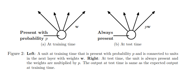
- Abstract:
- source:
- Ensembles of neural networks with different model configurations are known to reduce overfitting, but require the additional computational expense of training and maintaining multiple models.
- A single model can be used to simulate having a large number of different network architectures by randomly dropping out nodes during training.
- This is called dropout and offers a very computationally cheap and remarkably effective regularization method to reduce overfitting and improve generalization error in deep neural networks of all kinds.
- Large weights in a neural network are a sign of a more complex network that has overfit the training data.
- Probabilistically dropping out nodes in the network is a simple and effective regularization method.
- A large network with more training and the use of a weight constraint are suggested when using dropout.
- large NN:
- It is common for larger networks (more layers or more nodes) to more easily overfit the training data.
- When using dropout regularization, it is possible to use larger networks with less risk of overfitting. In fact, a large network (more nodes per layer) may be required as dropout will probabilistically reduce the capacity of the network.
- A good rule of thumb is to divide the number of nodes in the layer before dropout by the proposed dropout rate and use that as the number of nodes in the new network that uses dropout. For example, a network with 100 nodes and a proposed dropout rate of 0.5 will require 200 nodes (100 / 0.5) when using dropout.
- grid search parameters:
- Rather than guess at a suitable dropout rate for your network, test different rates systematically.
- weight constraint [= regularization, s. Dropout paper] [e.g.
maxnorm, L2, …] [Genaue Erklärung: s. Kapitel 5.1, 2. Absatz in Dropout paper]:- Network weights will increase in size in response to the probabilistic removal of layer activations. [?: Steht so nicht im paper. Eigentlich sollte Dropout einen regularizing effect haben, d.h. die weights shrinken.]
- Large weight size can be a sign of an unstable network.
- To counter this effect a weight constraint can be imposed to force the norm (magnitude) of all weights in a layer to be below a specified value.
- For example, the maximum norm constraint is recommended [im Dropout paper] with a value between 3-4.
- [Genaue Erklärung: s. Kapitel 5.1, 2. Absatz bis letzter Absatz in Dropout paper]
- eher Vermutungen als Erklärungen ?
- “A possible justification is that constraining weight vectors to lie inside a ball of fixed radius makes it possible to use a huge learning rate without the possibility of weights blowing up. The noise provided by dropout then allows the optimization process to explore different regions of the weight space that would have otherwise been difficult to reach. As the learning rate decays, the optimization takes shorter steps, thereby doing less exploration and eventually settles into a minimum.”
- eher Vermutungen als Erklärungen ?
- [Genaue Erklärung: s. Kapitel 5.1, 2. Absatz bis letzter Absatz in Dropout paper]
- For example, the maximum norm constraint is recommended [im Dropout paper] with a value between 3-4.
- large NN:
Classical 2nd order optimization methods
[source: LeCun et al. “Efficient BackProp”]
“Second order methods speed learning by estimating not just the gradient but also the curvature of the cost surface. Given the curvature, one can estimate the approximate location of the actual minimum.”
- Newton-Raphson Algorithm
- it is a $\mathcal{O}(N^3)$ (complexity of the matrix inversion of the $N\times N$ Hessian) method, where $N$ is the number of components of the parameter vector $\mathbf{w}$ [complexity of mathematical operations]
- see notes part 1
- Conjugate Gradient
- (1) it is a $\mathcal{O}(N)$ method,
- (2) it doesn’t use the Hessian explicitly,
- (3) it attempts to find descent directions that try to minimally spoil the result achieved in the previous iterations,
- (4) it uses a line search, and most importantly,
- (5) it works only for batch learning.
- Quasi-Newton (BFGS)
- (1) iteratively computes an estimate of the inverse Hessian,
- (2) is an $\mathcal{O}(N^2)$ algorithm,
- “Since the updates of the BFGS curvature matrix do not require matrix inversion, its computational complexity is only $\mathcal{O}(n^2)$, compared to $\mathcal{O}(n^3)$ in Newton’s method” - Wikipedia
- (3) requires line search and
- (4) it works only for batch learning.
- Gauss-Newton and Levenberg Marquardt algorithm
- (1) use the square Jacobi approximation,
- (2) are mainly designed for batch learning,
- (3) have a complexity of $\mathcal{O}(N^3)$ and
- (4) most important, they work only for mean squared error loss functions.