General RemarksPermalink

• Don’t lose sight of the bigger picture ! Only learn stuff when you need it !

As Feynman said: don’t read everything about a topic before starting to work on it. Think about the problem for yourself, figure out what’s important, then read the literature. This will allow you to interpret the literature and tell what’s good from what’s bad. - Y. LeCun

Overfitting problemPermalink

Why importantPermalink

TODO

EffectsPermalink

• larger $\mathbf{w}$ magnitudes

Paradoxes (related to the overfitting problem)Permalink

1. higher order polynomial contains all lower order polynomials as special cases
   • hence, the higher order polynomial is capable of generating a result at least as good as the lower order polynomial
     • d.h. das Polynom mit höherer Ordnung kann potentiell mindestens genauso gute Ergebnisse liefern ! Wieso passiert das nicht?
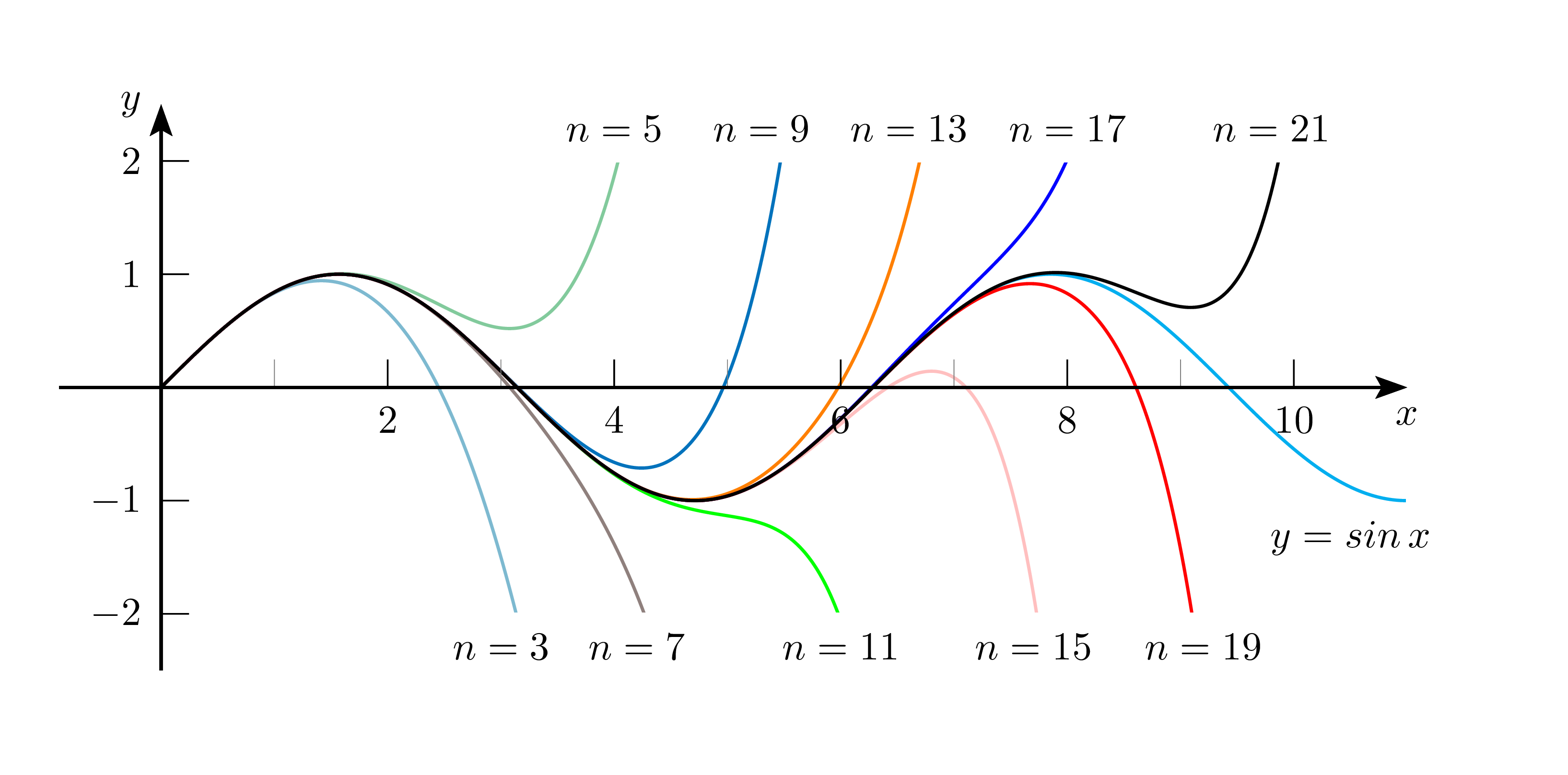
2. Sinus-Potenzreihe konvergiert für alle x in R und enthält Terme mit allen Potenzen von x (die geraden Potenzen haben Vorfaktor 0)

Aus 1. und 2. folgt, dass das Ergebnis mit jedem weiteren höheren x-Term prinzipiell umso genauer (d.h. näher an der ursprünglichen Sinusfunktion) werden könnte (weil die Potenzreihe ja auch mit jedem höheren x-Term genauer wird). Warum passiert das nicht?

Antwort:

1. Taylorreihe und linear model sind nicht vergleichbar: Die Taylor Reihe approximiert $\sin{x}$ und nicht die Datenpunkte. D.h. $E > 0$ für die Taylor Reihe, egal wie hoch die Ordnung des Taylor Polynoms ist! Aber das linear model kann mit hinreichend vielen $w_i$ stets einen perfekten Fit, i.e. $E=0$, erzielen.

2. Bei der Potenzreihe (Maclaurin Series) bleiben die weights der ersten N Terme fix, wenn man den Term der Ordnung N+1 hinzufügt, aber beim Fitten nicht ! Die Weights werden beim overfitting zu groß und sorgen für eine schlechtere representation der Targetfunktion als die Potenzreihenrepresentation der Targetfunktion, die die gleiche Ordnung hat!

   Deshalb muss man große weights “bestrafen” (d.h. einen penalty term einfügen aka regularizen), um die weights beim Fitten klein zu halten.

   Wir geben ja den weights völlige Freiheit, aber genau das ist das Problem: die weights fangen beim overfitting an auch den Noise in den Daten zu fitten, was für die hohen weight Werte sorgt!

   • Note: This happens with decision trees as well: the strongest variables are at the top of the tree, but at the very end, the split that the tree is making, might not be fitting signal but rather noise!

Possible Solutions (to the overfitting problem)Permalink

• Note: “regularization”, broadly speaking, means “constraining the universe of possible model functions”
• reduce number of model parameters (a form of regularization)
• increase number of data points $N$
  • i.e. reducing number of data points $N$ increases overfitting!
• increase regularization parameter $\lambda$ (in statistics: shrinkage methods)
  • Note: Do not include the bias term $w_0$ in the penalty term! Otherwise the procedure would depend on the origin chosen for the target.

    Note that often the coefficient $w_0$ is omitted from the regularizer because its inclusion causes the results to depend on the choice of origin for the target variable (Hastie et al., 2001), or it may be included but with its own regularization coefficient - Bishop_2006

    • see also here
  • $q=2$ in 3.29: quadratic regularization:
    • advantage: error function remains a quadratic function of $\mathbf{w}$ $\Rightarrow$ exact minimum can be found in closed form
    • terminology:
      • weight decay (in Deep Learning because in sequential learning algorithms, it encourages weight values to decay towards zero, unless supported by the data)
      • L2 regularization = parameter shrinkage = ridge regression (in statistics)
  • $q=1$ in 3.29: “lasso”
    • if $\lambda$ is sufficiently large, some of the coefficients are driven to $0$
      • leads to a sparse model in which the corresponding basis functions play no role
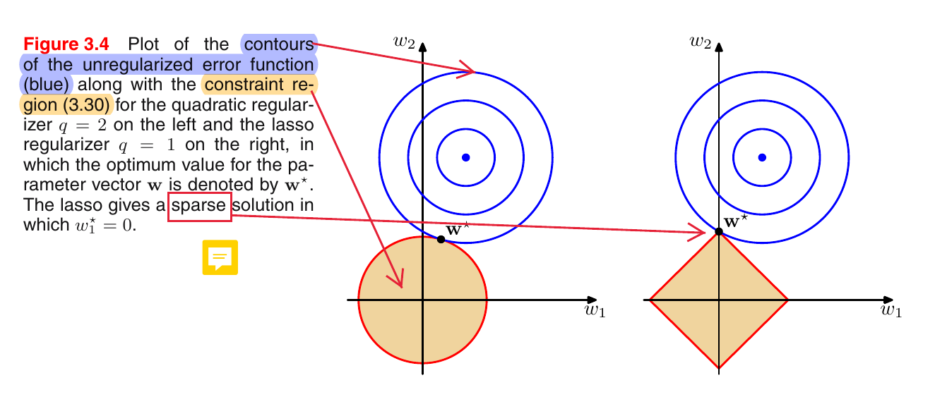
        • the origin of this sparsity can be seen here
          • increasing $\lambda$ corresponds to shrinking the yellow “constraint area”. The optimal parameter $\mathbf{w}^*$ corresponds to the point in the yellow area which is closest to the center of the blue circles (center = minimum of unregularized error function)
            • [Note: More generally, if the error function does not have circular contours, $\mathbf{w}^*$ would not necessarily be the “closest-to-center” point. In that case we would have to choose the point in the yellow area that minimizes the error function.]
          • the shape of these yellow “constraint areas” depends on $q$, but their size depends on $\lambda$
          • the blue circles only depend on the unregularized error function, i.e. changing $\lambda$ does not change the blue circles!
• use suitable heuristics (cf. overfitting MoGs)
• include a prior and find a MAP solution (equivalent to adding a regularization term to the error) [see below “Logistic Regression”]

Related ProblemsPermalink

In Maximum LikelihoodPermalink

BiasPermalink

• maximum likelihood approach systematically underestimates the true variance of the univariate Gaussian distribution (bias)
  • this is related to the problem of over-fitting (e.g. too many parameters in polynomial curve fitting):

    • $\mu_{ML}$ and $\sigma_{ML}^2$ are functions of $x_1, \ldots, x_N$
      • $\mu_{ML}=\frac{1}{N}\sum_{n=1}^N x_n$ and $\sigma^2{ML}=\frac{1}{N}\sum{n=1}^N (x_n - \mu_{ML})^2$
    • $x_1, \ldots, x_N$ come from a Gaussian distribution with (separate) $\mu$ and $\sigma^2$
      • see rules for sums of i.i.d. random variables (for $\mu$) and here (for $\sigma^2$)
    • one can show that the expectations of $\mu_{ML}$ and $\sigma_{ML}^2$ wrt this distribution are $\mathbb{E}[\mu_{ML}]=\mu$ and $\mathbb{E}[\sigma_{ML}^2]=\frac{N-1}{N}\sigma^2$, i.e. $\sigma_{ML}$ is biased and underestimates the true sample variance $\sigma$
    • Correcting for this bias yields the unbiased sample variance $\tilde{\sigma}^2=\frac{N}{N-1}\sigma_{ML}^2$

• increasing data size $N$ alleviates this problem (and reduces over-fitting [see above])
• this bias lies at the root of the over-fitting problem
• for anything other than small $N$ this bias is not a problem, in practice
• may become a problem for more complex models with many parameters, though

MoGPermalink

• singularities in the MoG likelihood will always be present (this is another example of overfitting in maximum likelihood)
  • Solution: use suitable heuristics
    • e.g. detect when a Gaussian component is collapsing and reset mean to a random value and reset covariance to some large value and then continue with the optimization

Logistic RegressionPermalink

• if the data set is linearly separable, ML can overfit
  • magnitude of $\mathbf{w}$ (which corresponds to the “slope” of the sigmoid in the feature space) goes to $\infty$
    • $\Rightarrow$ logistic sigmoid $\to$ Heaviside function
    • $\Rightarrow$ every point from each class $k$ is assigned posterior $P(C_k\vert\mathbf{x})=1$ (i.e. all posteriors are either $0$ or $1$ and there are no points with posteriors in between $0$ and $1$)
  • there is a continuum of such solutions
    • ML does not provide a way to favor one specific solution
    • which solution is found will depend on:
      • parameter initialization
      • choice of optimization algorithm
• Solution:
  • use a prior and find a MAP solution for $\mathbf{w}$
  • or equivalently: add a regularization term to the error function

Probability TheoryPermalink

Why important?Permalink

• **[Bayesian Inference](https://en.wikipedia.org/wiki/Bayesian_inference):** We have to understand the concepts of posterior and prior probabilities, as well as likelihood because e.g. both generative and discriminative linear models model the posterior probabilities $P(C_k\vert\mathbf{x})$ of the classes $C_k$ given the input $\mathbf{x}$.
  • when we minimize the error/loss function of a model, we are actually maximizing the likelihood
    • thus, e.g. Logistic Regression is a maximum likelihood method
      • Note: SVMs are non-probabilistic classifiers (have to use Platt scaling/calibration to make it probabilistic)

  “Bayesian inference is a method of statistical inference in which Bayes’ theorem is used to update the probability for a hypothesis as more evidence or information becomes available.” - Wikipedia

• **Probability distributions:**
  • Terminology:
    • probability distribution: overall shape of the probability density
    • probability density function, or PDF: probabilities for specific outcomes of a random variable
  • these are useful for:
    • Outlier detection: It is useful to know the PDF for a sample of data in order to know whether a given observation is unlikely, or so unlikely as to be considered an outlier or anomaly and whether it should be removed.
    • in order to choose appropriate learning methods that require input data to have a specific probability distribution.
    • for probability density estimation (see below).
    • distributions can form building blocks for more complex models (e.g. MoG)
• **Density estimation:** Sometimes we want to model the probability distribution $P(\mathbf{x})$ of a random variable $\mathbf{x}$, given a finite set $\mathbf{x}_1, \ldots, \mathbf{x}_N$ of observations (= density estimation).
  • there are infinitely many probability distributions that could have given rise to the observed data, i.e. the density estimation problem is fundamentally ill-posed
  • important because e.g. naive Bayes classifiers coupled with kernel density estimation (see below) can achieve higher accuracy levels.
  • 2 density estimation methods:
    • parametric density estimation:
      1. choose parametric distribution:
         • discrete random variables:
           • Binomial distribution
           • Multinomial distribution
         • continuous random variables:
           • Gaussian distribution
      2. Learning: estimate parameters of the chosen distribution given the observed data set
         • frequentist:
           • via Maximum Likelihood
         • Bayesian:
           1. introduce prior distributions over the parameters
           2. use Bayes’ theorem to compute the corresponding posterior over the parameters given the observed data
              • Note: This approach is simplified by conjugate priors. These lead to posteriors which have the same functional form as the prior. Examples:
              • conjugate prior for the parameters of the multinomial distribution: Dirichlet distribution
              • conjugate prior for the mean of the Gaussian: Gaussian
    • nonparametric density estimation:
      • size of the data set $N$ determines the form of the distribution, parameters determine the model complexity (i.e. “flexibility”, similar to the order of the polynomial in the polynomial curve fitting example) (but not the form of the distribution!)
      • histograms
      • nearest-neighbours (e.g. K-NN)
      • kernels (e.g. KDE)

Hence, understanding the basic concepts of probability theory is crucial for understanding linear models.

Sum rule, Product rule, Bayes’ TheoremPermalink

Example: Fruits in BoxesPermalink

• Let $P(B=r) = 0.4$ and $P(B=b) = 0.6$ (frequentist view: this is how many times the guy who picked the fruit picked each box [in the limit of infinitely many pickings], i.e. the picker had a tendency to pick the blue one more often).
  • Suppose that we pick a box at random, and it turns out to be the blue box. What’s the probability of picking an apple?
  • What’s the (overall) probability of choosing an apple?
  • Suppose we picked an orange. Which box did it come from?
• prior vs posterior explain intuitively (e.g. “evidence favouring the red box”)
• independence intuitively (e.g. “independent of which box is chosen”)

LikelihoodPermalink

• $P(\mathbf{x}\vert\vec{\theta})=L_{\mathbf{x}}(\vec{\theta})$ expresses how probable the observed data point $\mathbf{x}$ is (as a function of the parameter vector $\vec{\theta}$)
  • the likelihood is not a probability distribution over w, and its integral with respect to w does not (necessarily) equal one.
    • however, it is a probability distribution over x because integral w.r.t. $\mathbf{x}$ is $1$.
• MoGs: Similarly, in MoGs $P(\mathbf{x}\vert k)$ expresses the likelihood of $\mathbf{x}$ given mixture component $k$
  • i.e. the MoG likelihood itself is composed of several individual Gaussian likelihoods

Frequentist vs Bayesian approachPermalink

• there is no unique frequentist or Bayesian viewpoint

FrequentistPermalink

• Maximum Likelihood views true parameter vector $\theta$ to be unknown, but fixed (i.e. $\theta$ is not a random variable!).

BayesianPermalink

• In Bayesian learning $\theta$ is a random variable.
• prior encodes knowledge we have about the type of distribution we expect to see for $\theta$
  • (e.g. from calculations how fast the polar ice is melting)
• history:
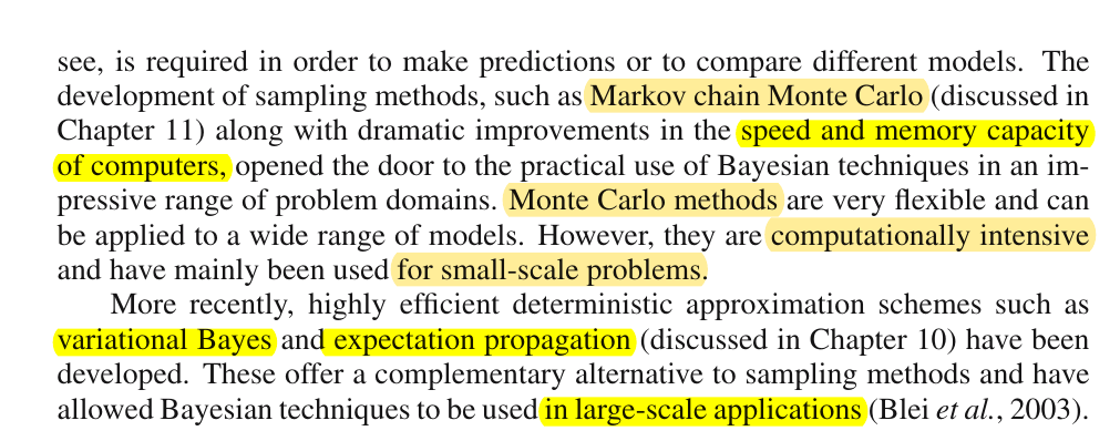
  • Bayesian framework has its origins in the 18th century, but the practical application was limited by “the difficulties in carrying through the full Bayesian procedure, particularly the need to marginalize (sum or integrate) over the whole of parameter space, which […] is required in order to make predictions or to compare different models” (Bishop)
    • technical developments changed this!
• critics:
  • prior distribution is often selected on the basis of mathematical convenience rather than as a reflection of any prior beliefs $\Rightarrow$ subjective conclusions
    • one motivation for so-called noninformative priors
    • Bayesian methods based on poor choices of prior can give poor results with high confidence
• advantages (compared to frequentist methods):
  • inclusion of prior knowledge
    • cf. example “tossing a coin three times and landing heads three times”:
      • Bayesian approach gives a better estimate of the probability of landing heads (whereas Maximum Likelihood would give probability 1)

The Uniform DistributionPermalink

• Mean: $\frac{(a+b)}{2}$ [derivation]
• Variance: $\frac{1}{12}(b-a)^2$ [derivation]

The Gaussian DistributionPermalink

EntropyPermalink

“Of all probability distributions over the reals with a specified mean $\mu$ and variance $\sigma^2$, the normal distribution $N(\mu,\sigma^2)$ is the one with maximum entropy.” - Wikipedia

• this also holds for the multivariate Gaussian (i.e. the multivariate distribution with maximum entropy, for a given mean and covariance, is a Gaussian)
  • Proof:
    • maximize the (differential) entropy of a distribution $p(x)$ $H[x]$ over all distributions $p(x)$ (likelihoods) subject to the constraints that $p(x)$ be normalized and that it has a specific mean and covariance
    • the maximum likelihood distribution is given by the multivariate Gaussian
• information (aka self-information, information content, self-entropy): $h_X(x)=-\log(p_X(x))$
• entropy
  • discrete: Shannon entropy $H(X)=-\sum p_X(x)\log p_X(x)$
    • equal to the expected information content of measurement of $X$: $\text{E}[h_X(x)]$
  • continuous: differential entropy $H(X)=-\int p_X(x)\log p_X(x)\text{dx}$

Central Limit Theorem (CLT)Permalink

Subject to certain mild conditions, the sum of a set of random variables (which is itself a random variable) has a distribution that becomes increasingly Gaussian as the number of terms in the sum increases.

• Let $X_1+\ldots+X_n$ be i.i.d. random variables. The expectation of $S_n=X_1+\ldots+X_n$ is $n\mu$ and the variance is $n\sigma^2$. [source]

Example: Sum of uniformly distributed i.i.d. random variables (e.g. distribution of the average of random variables)Permalink

$x_1,\ldots,x_N\sim \mathcal{U}[0,1]\xrightarrow[]{N \to \infty} \frac{1}{N}(x_1+\ldots +x_N)\sim\mathcal{N}(\frac{1}{2},\frac{1}{12N})$

• [Proof] for the mean $\frac{1}{2}$ and the variance $\frac{1}{12N}$, where $\bar{X}=\frac{1}{N}(x_1+\ldots +x_N)$ [source]
  • Recall the rules for expectations and variances.
• Notation: The $[0,1]$ in $\mathcal{U}[0,1]$ denotes an interval, whereas the $(\frac{1}{2},\frac{1}{12N})$ in $\mathcal{N}(\frac{1}{2},\frac{1}{12N})$ denotes the mean and the variance of the Gaussian (specifying an interval for the Gaussian does not make sense)

Relation to other distributionsPermalink

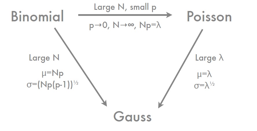
• Binomial distribution $\xrightarrow[]{N\to\infty}$ Gaussian distribution

Well-definedPermalink

• the Gaussian is well-defined in all dimensions only if $\Sigma$ is positive definite (ie all Eigenvalues are strictly positive)
  • if at least one of the Eigenvalues is zero, then the distribution is singular and confined to a subspace of lower dimensionality
  • Definiteness is commonly (i.e. for most authors) only defined for symmetric matrices (see Definiteness)

Intuition for Multivariate GaussiansPermalink

• apply spectral decomposition of the covariance $\Sigma$
  • Note: spectral decomposition is the Eigendecomposition of a normal or real symmetric matrix (see Eigendecomposition)
  • Under which conditions is a spectral decomposition possible?
    • spectral theorem: “If $A$ is Hermitian, then there exists an orthonormal basis of $V$ consisting of eigenvectors of $A$. Each eigenvalue is real.”
      • “Hermitian” is a generalization of “symmetric” for complex matrices
      • since $\Sigma$ is symmetric w.l.o.g. (see below), we can apply the spectral theorem
• Shape of the Gaussian:
  • scaling given by $\lambda_i$,
  • shifted by $\mathbf{\mu}$,
  • rotation given by the eigenvectors $\mathbf{u}_i$
• new coordinate system defined by eigenvectors $\mathbf{u}_i$ with axes $y_i=\mathbf{u}_i^T(\mathbf{x}-\mathbf{\mu})$ for $i=1,\ldots,D$

  “In linear algebra, eigendecomposition is the factorization of a matrix into a canonical form, whereby the matrix is represented in terms of its eigenvalues and eigenvectors. Only diagonalizable matrices can be factorized in this way. When the matrix being factorized is a normal or real symmetric matrix, the decomposition is called “spectral decomposition”, derived from the spectral theorem.” - Wikipedia

  • origin of new coordinate system is at $\mathbf{y}=\mathbf{0}$, i.e. at $\mathbf{x}=\mathbf{\mu}$ in the old coordinate system!
• Normalization: one can show that i.e. in the EV coordinate system the joint PDF factorizes into $D$ independent univariate Gaussians! The integral is then $\int{p(\mathbf{y})d\mathbf{y}}=1$, which shows that the multivariate Gaussian is normalized.
• 1st order and 2nd order moments:
  • Note: 2nd order moment (i.e. $\mu\mu^T+\Sigma$) $\neq$ covariance of $\mathbf{x}$ (i.e. $\Sigma$)

Number of Parameters of Gaussian ModelsPermalink

• Number of independent parameters: $\Sigma$ has in general $D(D+1)/2$ independent parameters

  • $D^2-D$ non-diagonal elements of which $(D^2-D)/2$ are unique
  • $D$ diagonal elements
  • i.e. in total $(D^2-D)/2+D=D(D+1)/2$ independent parameters in $\Sigma$

  • grows quadratically with $D$ $\Rightarrow$ manipulating/inverting $\Sigma$ can become computationally infeasible for large $D$
  • $\Sigma$ and $\mu$ together have $D(D+3)/2$ independent parameters
• special cases of covariance matrices (also counting $\mu$):
  • general $\qquad\qquad\qquad\qquad\Rightarrow D(D+3)/2$ independent parameters (shape: hyperellipsoids)
  • diagonal $\Sigma=\mathop{\mathrm{diag}}(\sigma_i)$ $\qquad\Rightarrow 2D$ independent parameters (shape: axis-aligned hyperellipsoids)
    • $\Leftrightarrow \text{cov}(X,Y)=0$ for all non-diagonal elements
    • $\Leftrightarrow$ Random Variables uncorrelated
    • $\Leftrightarrow$ Random Variables independent
    • Warning: The words uncorrelated and independent may be used interchangeably in English, but they are not synonyms in mathematics. Independent random variables are uncorrelated, but uncorrelated random variables are not always independent. source
  • isotropic $\Sigma=\sigma^2\mathbf{I}$ $\qquad\qquad\Rightarrow D+1$ independent parameters (shape: hyperspheres)

Conditionals and Marginals of GaussiansPermalink

• Conditionals and Marginals of Gaussians are again Gaussians

Limitations of GaussiansPermalink

ProblemPermalink

• as discussed above, the Gaussian can be both
  • too flexible (too many parameters) and
  • too limited in the distributions that it can represent
    • Gaussian is unimodal, i.e. it has a single maximum, but we want to approximate multimodal distributions!

Solution: Latent variable modelsPermalink

• use latent (hidden, unobserved) variables
  • discrete latent variables $\Rightarrow$ MoGs (which are multimodal!)
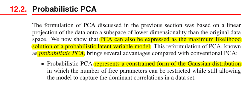
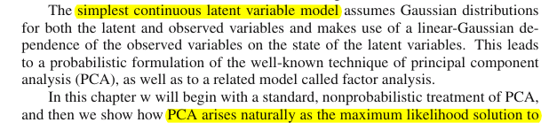
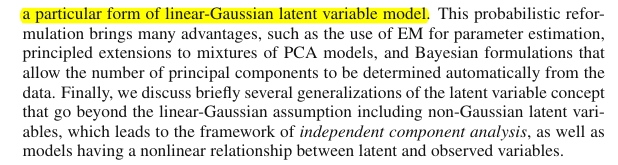
  • continuous latent variables $\Rightarrow$ “probabilistic PCA”, factor analysis

    “Probabilistic PCA represents a constrained form of the Gaussian distribution in which the number of free parameters can be restricted while still allowing the model to capture the dominant correlations in a data set.” - Bishop, “Pattern Recognition and Machine Learning”

    • i.e., like MoGs, probabilistic PCA is a parametric density estimation method (see above)
    • see also here and here
    • probabilistic PCA and factor analysis are related
    • formulation of PCA as a probabilistic model was proposed independently by Tipping and Bishop (1997, 1999b) and by Roweis (1998) $\rightarrow$ see “Linear Gaussian Models”
      • also important applications in control theory
    • [paper: GMMs vs Mixtures of Latent Variable Models]

      “One of the most popular density estimation methods is the Gaussian mixture model (GMM). A promising alternative to GMMs [= MoGs] are the recently proposed mixtures of latent variable models. Examples of the latter are principal component analysis and factor analysis. The advantage of these models is that they are capable of representing the covariance structure with less parameters by choosing the dimension of a subspace in a suitable way. An empirical evaluation on a large number of data sets shows that mixtures of latent variable models almost always outperform various GMMs both in density estimation and Bayes classifiers.” - from [paper: GMMs vs Mixtures of Latent Variable Models]

• Latent variable models:
  • discrete latent variables
    • continuous $\mathbf{x}$:
      • MoG/GMM
    • discrete $\mathbf{x}$:
      • Mixture of Bernoulli distributions
  • continuous latent variables
    • probabilistic PCA
    • factor analysis

Proof: Covariance $\Sigma$ symmetric w.l.o.g.Permalink

see [proof-Gaussian-cov-symmetric-wlog]

• Key point: If $\mathbf{A}=\mathbf{\Sigma}^{-1}$ is not symmetric, then there is another symmetric matrix $\mathbf{B}$ so that $\Delta^2=(\mathbf{x}-\mathbf{\mu})^T\mathbf{\Sigma}^{-1}(\mathbf{x}-\mathbf{\mu})$ is equal to $\Delta^2=(\mathbf{x}-\mathbf{\mu})^T\mathbf{B}(\mathbf{x}-\mathbf{\mu})$.
• Why is this important?
  • If $\Sigma$ was not symmetric, its eigenvectors would not necessarily form an orthonormal basis. Hence, the above intuition for the Gaussians would not hold.
  • If $\Sigma$ is a real, symmetric matrix its eigenvalues are real and its eigenvectors can be chosen to form an orthonormal basis (symmetric matrices/diagonalizable and symmetric matrices/orthoganally diagonalizable)
    • in other words, it’s important in order to apply the spectral theorem:

      “The finite-dimensional spectral theorem says that any symmetric matrix whose entries are real can be diagonalized by an orthogonal matrix. More explicitly: For every real symmetric matrix $A$ there exists a real orthogonal matrix $Q$ such that $D = Q^{\mathrm{T}} A Q$ is a diagonal matrix. Every real symmetric matrix is thus, up to choice of an orthonormal basis, a diagonal matrix.” - Wikipedia

MoG/GMMPermalink

• Motivation:
  • The K-means (hard-assignments) and the EM algorithm (soft-assignments) result from Maximum Likelihood estimation of the parameters of MoGs.
• MoGs are probabilistic generative models (see below), if we view each mixture component $k$ as a class
• parameters are determined by:
  • Frequentist:
    • Maximum Likelihood:
      • problem 1: no closed-form analytical solution
        • solutions:
          • iterative numerical optimization
            • gradient-based optimization
          • EM algorithm
      • problem 2: maximization of MoG likelihood is not a well posed problem because “singularities” will always be present (for both the univariate and the multivariate case, but not for a single Gaussian!)
        • solution:
          • see section Overfitting in Maximum Likelihood
      • problem 3: “identifiability”: $K!$ equivalent solutions
        • important issue when we want to interpret the parameter values
        • however, not relevant for density estimation
      • problem 4: number of mixture components fixed in advance
        • solution: variational inference (see below)
  • Bayesian:
    • Variational Inference
      • little additional computation compared with EM algorithm
      • resolves the principle difficulties of maximum likelihood
      • allows the number of components to be inferred automatically from the data
• can be written in two ways:
  • standard formulation
  • latent variable formulation [9.10-12] (see section [MoG_latent_var])
    • why useful?
      • for ancestral sampling (siehe Zettel)
      • simplifications of the ML solution of MoG: we can work with the joint distribution $P(\mathbf{x},\mathbf{z})$ instead of the marginal $P(\mathbf{x})$ $\Rightarrow$ we can write the complete-data log-likelihood in the form [9.35]
        • simplifies maximum likelihood solution of MoG
          • using latent variables the complete-data log-likelihood can be written as [9.35], which is basically $p(\mathbf{X},\mathbf{Z})=\prod_{n=1}^N p(\mathbf{z}_n)p(\mathbf{x}_n\vert\mathbf{z}_n)$ (recall: there is one $\mathbf{z}_n$ for each $\mathbf{x}_n$)
            • do not sum over $\mathbf{z}$ as in [9.12]! 9.12 is $p(\mathbf{x})$ and not $p(\mathbf{x},\mathbf{z})$! Simply insert [9.10] and [9.11] in $p(\mathbf{X},\mathbf{Z})$.
            • this leads to a closed form solution for the MoG maximum likelihood (which is useless in practice, though)
              • maximization w.r.t. mean and covariance is exactly as for the single Gaussian, except that it involves only the data points that are assigned to each component. The mixing coefficients are equal to the fractions of data points assigned to the corresponding components.
                • this simplification would not be possible without the introduction of latent variables!
              • however, the latent variables are not known, in practice
                • but we can maximize the expectation of the complete-data log likelihood function (w.r.t. the posterior distribution of the latent variables) [9.40]
                  • we can calculate this expectation by choosing some initial parameters in order to calculate $\gamma(z_{nk})$ and then maximizing [9.40] w.r.t. the parameters (while keeping the responsibilities fixed)
                  • $\Rightarrow$ EM algorithm
            • Note: the MoG likelihood without latent variables (see 9.14) cannot be maximized in closed form, but the EM algorithm gives closed form expressions for $\mu_k$, $\Sigma_k$ and $\pi_k$.
              • (“closed form expression” only means “a mathematical expression that uses a finite number of standard operations” and hence, $\mu_k$, $\Sigma_k$ and $\pi_k$ are in closed form)
            • Interpreting [9.36] is much easier than interpreting 9.14!
              • maximization wrt a mean or a covariance:
                • in 9.36: $z_{nk}$ “filtert” die Punkte, die zu Component $\mathcal{N}_k$ assigned wurden, ansonsten alles wie bei ML bei einem single Gaussian

Mixture Models in generalPermalink

• use cases:
  • framework for building more complex probability distributions
  • clustering data
    • clustering with hard assignments (K-means algorithm)
    • clustering with soft assignments (EM algorithm)

Applications of Mixture ModelsPermalink

• applications typically model the distribution of pixel colors and learn a MoG to represent the class-conditional densities:
  • image segmentation
    • mark two regions to learn MoGs and classify background VS foreground
  • tracking
    • train background MoG model with an empty scene (i.e. the object to be tracked is not in this scene at first) in order to model common appearance variations for each pixel
    • anything that cannot be explained by this model will be labeled as foreground, i.e. the object to be tracked
    • Note: in order to adapt to e.g. lighting changes the MoG can be updated over time

Non-parametric ModelsPermalink

Proof: Convergence of the KNN and KDE EstimatesPermalink

• problem: Why is the approximation $p=\frac{K}{NV}$ justified?
• Aus Bishop_2006:
  • “It can be shown that both the K-nearest-neighbour density estimator and the kernel density estimator converge to the true probability density in the limit $N\to\infty$ (provided $V$ shrinks suitably with $N$, and $K$ grows with $N$)”
    • Aus Duda, Hart 1973:
      • $p_n$ ist das n-th estimate für die wahre PDF $p$
        • $\mathcal{R}_n$ ist eine Folge von Regionen, die das $\mathbf{x}$ enthalten
        • $V_n$ ist das Volumen von $\mathcal{R}_n$
        • $k_n$ ist die Anz. an Samples, die in $\mathcal{R}_n$ fallen
        • Achtung: $n$ ist sowohl Folgenindex als auch die Gesamtzahl der i.i.d. drawn Samples!
      • die $\mathcal{R}_n$ bilden eine Folge
      • zu jedem $\mathcal{R}_n$ gibt es ein $p_n$
      • man kann zeigen, dass $p_n$ gegen das wahre $p$ konvergiert, wenn:
      • “There are two common ways of obtaining sequences of regions that satisfy these conditions” - Duda, Hart 1973
        • Parzen window (KDE)
        • K-NN
      • d.h. KDE und K-NN sind beides Methoden, um solche $p_n$ zu konstruieren, die diesen Bedingungen genügen

K-NNPermalink

• $k=1$: decision boundary = hyperplanes that form perpendicular bisectors of pairs of points from different classes
• Ties can be broken at random

Outlier removalPermalink

• by choosing a suitable nonlinearity (e.g. sigmoid, tanh)
  • cf. least-squares discriminant example
• remove outlier data point completely from the data set

Model Selection / ComparisonPermalink

• TODO

The Curse of DimensionalityPermalink

Why important?Permalink

• For all classifiers, the more dimensions we have in the input space (= feature space), the more training data we need.
  • Consider the simple classifier described in Bishop, Chapter 1.4 “The Curse of Dimensionality”.
    • The problem with an exponentially large number of cells in the input space is that we would need an exponentially large number of training data points in order to ensure that the cells are not empty. Therefore, applying this classifier to more input variables (here: only two input variables (= features): $x_6$ and $x_7$) becomes infeasible.

“In machine learning problems […] typically an enormous amount of training data is required to ensure that there are several samples with each combination of values. A typical rule of thumb is that there should be at least 5 training examples for each dimension in the representation. […] This [“Curse of Dimensionality”] phenomenon states that with a fixed number of training samples, the average (expected) predictive power of a classifier or regressor first increases as the number of dimensions or features used is increased but beyond a certain dimensionality it starts deteriorating instead of improving steadily.” - Wikipedia

• TODO

Decision TheoryPermalink

Why important?Permalink

The classification problem can be broken down into two stages:

• Inference Stage: use training data to learn a model for $P(C_k\vert\mathbf{x})$
• Decision Stage: use these $P(C_k\vert\mathbf{x})$ to make optimal class assignments

Generative and discriminative models use this “two stage” approach. Discriminant functions do not have access to the posteriors $P(C_k\vert\mathbf{x})$!

ML for Mixture ModelsPermalink

K-means algorithmPermalink

• corresponds to a particular nonprobabilistic limit of EM applied to MoGs (see EM algorithm)
• goal: find values for all $r_{nk}$ and $\pmb{\mu}_k$ so as to minimize $J$ (= “sum of all distances”)

K-means intuitivelyPermalink

• E step: determine all $r_{nk}$ (“assign $\mathbf{x}_n$ to closest cluster center”)
• M step: determine all $\pmb{\mu}_k$ (“set $\pmb{\mu}_k$ equal to the mean of all $\mathbf{x}_n$ assigned to cluster $k$”)
• Note: this algorithm is guaranteed to reduce the value of the objective function $J$ in each phase and hence, is guaranteed to converge after a finite number of iterations
  • $J$ corresponds to the negative expectation of the complete-data log likelihood in the EM algorithm, see 9.43 and disussion of general EM algorithm

Initialization of K-meansPermalink

• choose the initial $\pmb{\mu}_k$ to be equal to a random subset of $K$ data points

AdvantagesPermalink

• simple and fast to compute
• guaranteed convergence in finite number of iterations
  • convergence faster than for standard EM algorithm

Issues in practicePermalink

• may converge to a local rather than global minimum (like the EM algorithm)
• the final result depends on initialization
• E step may be slow $\mathcal{O}(KN)$ ($K$: number of means, $N$: number of data points) because it requires computing all distances
  • solution: speed up by
    • precompute a data structure (e.g. a tree, where nearby points are in same subtree)
    • avoid unnecessary distance calculations (e.g. using the triangle inequality)
• detects spherical clusters only
• sensitive to outliers
• choosing $K$

Online versionPermalink

• above a batch version of K-means is described, but there is also a sequential update online version
• via Robbins-Monro procedure (MacQueen, 1967)
  • see Bishop, 2.3.5 “Sequential estimation”

K-medoids algorithmPermalink

• uses other dissimilarity measure $\mathcal{V}$
  • hence, its M step is potentially more complex
    • solution: restrict each cluster prototype to be equal to one of the $\mathbf{x}_n$ assigned to that cluster
      • in this case: $\mathcal{O}(N_k^2)$ evaluations of $\mathcal{V}(.,.)$ ($N_k$: number of points assigned to cluster k)
• advantages compared to K-means:
  • cluster means are more robust to outliers
  • limits the data types that can be considered
    • e.g. for categorical inputs a Euclidean distance cannot be calculated

ComplexityPermalink

• E step: $\mathcal{O}(KN)$ (for both K-means and K-medoids)
• M step: $\mathcal{O}(N_k^2)$ for each cluster $k$

Elliptical K-meansPermalink

• idea: EM gives an estimate for $\Sigma$, however, standard K-means (which is a special case of an EM algorithm) does not estimate $\Sigma$
  • $\Rightarrow$ hard assignments with general $\Sigma$ instead of isotropic $\Sigma=\epsilon\mathbf{I}$ for $\epsilon\to 0$ (Sung, Poggio, 1994)

Applications of K-meansPermalink

• Image Segmentation
• Image Compression
  • using vector quantization

Latent variable formulation of Mixture DistributionsPermalink

• this is basically an alternative (i.e. equivalent) formulation of mixture models (e.g. MoGs) that simplifies certain calculations (see e.g. “latent variable view of EM algorithm”)
• Merke: "For every observed data point $\mathbf{x}_n$ there is a corresponding latent variable $\mathbf{z}_n$."
  • i.e. there are $N$ latent variables $\mathbf{z}_n$, so to speak
  • $\mathbf{z}_n$ is not known
    • in ancestral sampling $\mathbf{z}$ is known because we sample from $P(\mathbf{z})$ first, so we know the value of $\mathbf{z}$
      • and, therefore, we know the component that generates $\mathbf{x}$
        • corresponding to the $z_k$ which is equal to $1$
  • $\mathbf{z}_n$ encodes which mixture component $\mathbf{x}_n$ belongs to
• ${\mathbf{X},\mathbf{Z}}$ is called complete data set
  • the corresponding log-likelihood is $\ln P(\mathbf{X},\mathbf{Z}\vert\mathbf{\vec{\theta}})$, where $P(\mathbf{X},\mathbf{Z}\vert\mathbf{\vec{\theta}})=\prod_{n=1}^N P(\mathbf{z}_n)P(\mathbf{x}_n\vert\mathbf{z}_n)$
    • this is basically a generalization of $\ln P(\mathbf{X}\vert\mathbf{\vec{\theta}})$ which simplifies the Maximum Likelihood treatment for MoGs (in theory, not in practice, see theoretical ML for MoG)
• actual observed data $\mathbf{X}$ is called incomplete
• can be interpreted as defining assignments of data points to specific components of the mixture

EM algorithmPermalink

• goal: find maximum likelihood solutions for models having latent variables

ApplicationsPermalink

• use cases:
  • find MAP solutions for models in which a prior $P(\mathbf{\vec{\theta}})$ is defined
  • Handling missing values: the EM algorithm can also be applied when the unobserved variables $\mathbf{z}$ correspond to missing values in the data set
    • only applicable, if values are missing at random (MAR)

      “Under the classical missing at random mechanism (MAR) assumption, the parameters can thus be estimated by maximizing the observed likelihood. To do so, it is possible to use an Expectation-Maximization (EM) algorithm (Dempster, Laird, and Rubin, 1977) […].” - source: section 11.1.1.3 Two recommended methods: EM / Multiple imputation

    • see probabilistic PCA

      “Because we now have a fully probabilistic model for PCA, we can deal with missing data, provided that it is missing at random, by marginalizing over the distribution of the unobserved variables. Again these missing values can be treated using the EM algorithm. We give an example of the use of this approach for data visualization in Figure 12.11.” - Bishop_2006

General EM AlgorithmPermalink

• E step:
  • find $P(\mathbf{Z}\vert\mathbf{X},\pmb{\theta}^{old})$
    • in the standard EM algorithm this corresponding to: find $\gamma(z_{nk})$
  • find the expectation (w.r.t this $P(\mathbf{Z}\vert\mathbf{X},\pmb{\theta}^{old})$) of the complete-data log likelihood $Q(\pmb{\theta},\pmb{\theta}^{old})$
• M step: update $\pmb{\theta}^{new}=\text{arg max}_{\pmb{\theta}}Q(\pmb{\theta},\pmb{\theta}^{old})$
• Note: this algorithm is guaranteed to increase the incomplete-data log likelihood in each cycle

Initialization of EMPermalink

1. Run K-means (e.g. M times)
2. pick the best result (i.e. lowest error $J$)
3. initialize EM parameters:
   • initialize $\Sigma_k$ to $\Sigma$ of clusters found by K-means
   • initialize $\pi_k$ to fraction of $\mathbf{x}$ assigned to clusters found by K-means

Issues in practicePermalink

• MoG singularities: employ techniques to avoid singularities (see overfitting MoGs)
• multiple local maxima: the log likelihood has in general multiple local maxima
  • the EM algorithm is not guaranteed to converge to the largest maximum!

Credit Assignment problemPermalink

• problem: when we are given $\mathbf{x}_n$, we don’t know which component generated this point
• solution: we can calculate the responsibilities of each component for explaining $\mathbf{x}n\gamma_k(\mathbf{x}_n)=\gamma(z{kn})=p(z_k=1\vert\mathbf{x}_n)$
  • corresponds to a soft assignment of each sample $\mathbf{x}_n$ to a mixture component $\Rightarrow$ this is why the EM algorithm is sometimes referred to as “Clustering with soft assignments”
    • $\mathbf{x}_n$ is assigned to all mixture components (with some probability $\gamma_k(\mathbf{x}_n)$ for each component) instead of only one component (cf. hard assignments of the K-means algorithm)
  • This is what the E-step of the EM algorithm does!

Relation to K-meansPermalink

• corresponds to a particular nonprobabilistic limit of EM applied to MoGs
  • consider a MoG where each mixture component has covariance $\epsilon\mathbf{I}$ and thus looks like [9.41]
    • then the responsibilities $\gamma(z_{nk})$ for a data point $\mathbf{x}$ all go to zero except for one which will go to unity (in other words: $\gamma(z_{nk})\to r_{nk}$)
      • this corresponds to a hard assignment of the data point $\mathbf{x}_n$
    • the $\pmb{\mu}_k$ will go to the K-means $\pmb{\mu}_k$
    • the $\pi_k$ will be reset to the fraction of data points assigned to cluster $k$ (as usual in the EM algorithm)
      • however, the $\pi_k$ are irrelevant for the algorithm now
    • the expected complete-data log likelihood $Q(\pmb{\theta},\pmb{\theta}^{old})$ will go to the negative of the distortion measure $J$ for the K-means algorithm

Linear models for regressionPermalink

• the polynomial is one example of a broad class of functions called linear regression models
• linear regression models:
  • are always linear functions of the parameters

Linear models for classificationPermalink

Linear Models vs MLPsPermalink

Difference to DNNs/MLPs: linear models use fixed basis functions, whereas DNNs/MLPs use learned basis functions [via hidden layers]

Linear Models vs Generalized Linear ModelsPermalink

• linear models (i.e. WITHOUT activation function)
  • these models are linear in the parameters!
  • the decision surfaces are linear functions of the input vector $\mathbf{x}$ (or of the feature vector $\pmb{\phi}(\mathbf{x})$, see LBFs)
    • ($D-1$-dimenstional hyperplanes)
• generalized linear models (i.e. WITH activation function)
  • these models are not linear in the parameters!
    • (in cotrast to the linear models for regression discussed in Bishop_2006)
  • the decision surfaces are linear functions of the input vector $\mathbf{x}$ (or of the feature vector $\pmb{\phi}(\mathbf{x})$, see LBFs)
    • ($D-1$-dimenstional hyperplanes)
    • because decision surfaces correspond to $y(\mathbf{x})=\text{const}$, which implies $\mathbf{w}^\top\mathbf{x}+w_0=\text{const}$
  • Open Questions:
    • lecture slides: if the activation function is not monotonous, the decision surface is not a linear function of $\mathbf{x}$, why?
  • why decision surfaces plural and not singular?

discriminant functionsPermalink

Note: Bishop_2006 only discusses linear discriminants in chapter 4.1 (i.e. the decision surfaces are $D-1$-dimensional hyperplanes) which does not mean that discriminant functions must always be linear! In particular,

• the introduction to chapter 4 mentions that all algorithms discussed in this chapter are equally applicable using nonlinear transformations $\pmb{\phi}$.
• this is also mentioned in chapter “4.3.1 Fixed basis functions”

• 2 classes
  • single 2-class discriminant $y(\mathbf{x})=\mathbf{w}^\top\mathbf{x}+w_{0}$
  • equivalently: single 2-class discriminant comprising $2$ linear functions $y_k(\mathbf{x})=\mathbf{w}^\top_k\mathbf{x}+w_{k0}$
  • Rosenblatt’s perceptron
• K classes
  • one-vs-rest
  • one-vs-one
  • single K-class discriminant comprising $K$ linear functions $y_k(\mathbf{x})=\mathbf{w}^\top_k\mathbf{x}+w_{k0}$
    • decision regions are convex (proof in Bishop_2006)
      • “Every convex subset of $\mathbb{R}^n$ is simply [= singly] connected.” - Wikipedia
        • $\Rightarrow$ decision regions are also singly connected
• learning the parameters
  • least squares
    • (see Bishop_2006, 1.2.5)
      • wrong tool for binary (i.e. 1-of-K coded) targets because binary targets do not have a Gaussian distribution and least squares (1.67) corresponds to ML under the assumption of a “Gaussian conditional distribution for $t$ given $x$ given by (1.60)” [quote from Fig. 1.16 Bishop_2006] $p(t\vert x)$
  • Fisher’s linear discriminant
  • perceptron algorithm, i.e. Gradient Descent
  • Gradient Descent

probabilistic generative models (indirect modeling of posterior)Permalink

source

• Examples:
  • MoGs
• $P(C_k\vert\mathbf{x})$ can be written as logistic sigmoid 4.57
  • i.e. $P(C_k\vert\mathbf{x})$ has a sigmoidal shape (when viewed as function of $\mathbf{x}$), if “$a$” 4.58 is linear in $\mathbf{x}$!
• first model $P(\mathbf{x}\vert C_k)$ and $P(C_k)$, then use 4.57-4.58 to find $P(C_k\vert\mathbf{x})$ (or use equivalently Bayes’ theorem 1.82 and 1.83)
  • Examples:
    • Continuous Inputs: (Gaussian distribution)
      • model each $P(\mathbf{x}\vert C_k)$ as a Gaussian 4.64, where all classes share the same $\pmb{\Sigma}$ $\Rightarrow$ posterior $P(C_k\vert\mathbf{x})$ is the logistic sigmoid 4.65 (2 classses) or the softmax 4.62 ($K\geq2$ classes) where $a_k$ is given by 4.68, i.e. a generalized linear model
        • (i.e. linear decision boundaries, but not linear in parameters!)
        • decision boundaries are where (the 2 largest) posteriors are equal
        • use Maximum Likelihood to determine parameters of Gaussian 4.64 and priors $P(C_k)$ (requires data set)
        • priors enter only through $w_0$ 4.67
          • i.e. priors shift the decision boundary parallelly (vgl. 4.65 mit distance from the origin to the decision surface 4.5)
          • i.e. priors shift the parallel contours of constant posterior probability
        • the argument of the sigmoid (2 classes) or the $a_k(\mathbf{x})$ of the softmax ($K\geq2$ classes) are linear functions of the inputs $\mathbf{x}\Leftrightarrow$ class conditionals $P(\mathbf{x}\vert C_k)$ are members of the exponential family
        • Note: if the classes do not share the same $\pmb{\Sigma}$, the decision boundaries will be quadratic, i.e. the $P(C_k\vert\mathbf{x})$ are not governed by a generalized linear model!
    • Discrete Inputs: (Bernoulli distribution)
      • model $P(\mathbf{x}\vert C_k)$ as Bernoulli naive Bayes model $P(\mathbf{x}\vert C_k)=\prod_{i=1}^Dp_{ki}^{x_i}(1-p_{ki})^{(1-x_i)}$ $\Rightarrow$ posterior $P(C_k\vert\mathbf{x})$ a logistic sigmoid (2 classses) or the softmax 4.62 ($K\geq2$ classes) where $a_k$ is given by 4.82, i.e. again a generalized linear model
        • $x_i\in{0,1}$ (e.g. “spam or ham”)
        • $p_{ki}$ is the probability of class $C_k$ generating the term $x_i$
        • $a_k(\mathbf{x})$ are again linear functions of the inputs $x_i$
        • also holds for discrete variables with $M>2$ states
        • App: popular for document classification tasks
    • Exponential Family:
      • above results are special cases: If class-conditional densities are members of the exponential family, the posterior $P(C_k\vert\mathbf{x})$ is a logistic sigmoid (2 classses) with argument 4.85 or the softmax 4.62 ($K\geq2$ classes) where $a_k$ is given by 4.86, i.e. again a generalized linear model

probabilistic discriminative models (direct modeling of posterior)Permalink

source

• maximize likelihood function defined through $P(C_k\vert\mathbf{x})$
  • fewer adaptive parameters to be determined than for generative models
    • zB. $M$ parameters for logistic regression vs. $M (M + 5) / 2 + 1$ for Gaussian generative model approach as described above, which grows quadratically with $M$
  • may lead to better predictive performance than generative models, particularly when the $P(\mathbf{x}\vert C_k)$ assumptions of the generative models are not accurate
  • Examples:
    • logistic regression (2 classes)
    • softmax regression/multiclass logistic regression (multiple classes)

generative vs discriminative modelsPermalink

• Generative methods model the joint probability distribution over observation and label sequences, whereas discriminative methods directly model the decision boundary
• Wikipedia “Generative model”:
  • Terminology is inconsistent, but three major types can be distinguished, following Jebara (2004):
    1. A generative model is a statistical model of the joint probability distribution $P ( X , Y )$ on given observable variable $X$ and target variable $Y$;
    2. A discriminative model is a model of the conditional probability $P ( Y \vert X = x )$ of the target $Y$, given an observation $x$; and
    3. Classifiers computed without using a probability model are also referred to loosely as “discriminative”.
• Generative models:
  • can deal naturally with missing data
  • can handle sequences of varying length (hidden Markov models)
  • examples:
    • Linear discriminant analysis (LDA) (a generalization of Fisher’s linear discriminant)
    • naive Bayes classifier
• Discriminative models:
  • generally give better performance on discriminative tasks than generative models
  • examples:
    • logistic regression
• Combining both:
  • using kernels: Bishop_2006 (6.28) ff.
    1. use generative model to define a kernel
    2. use this kernel in a discriminative approach
  • Laserre_2006

Linear Basis Function ModelsPermalink

• decision boundaries are linear in feature space ($\pmb{\phi}$ space), but nonlinear in input space ($\mathbf{x}$ space)
• Note: nonlinear transformations $\pmb{\phi}$:
  • cannot remove class conditional densities’ overlap (i.e. region where posteriors are not $0$ or $1$) !
  • they can even increase the level of overlap !
  • they can also create overlap where none existed !

Least Squares and Maximum LikelihoodPermalink

• S. 141: maximization of likelihood function under a conditional Gaussian (target vector 3.7) noise distribution 3.8 for a linear model is equivalent to minimizing a sum-of-squares error function

Relation of Gradient Descent to Taylor ExpansionPermalink

• see chapter 3.1-3.2

Delta rulePermalink

• Rule: $\frac{\partial E_n}{\partial \mathbf{w}}=$ ‘error’ (aka Delta) $y_n-t_n$ times the feature vector $\vec{\phi}_n$
  • $E_n$: contribution to the error function from a data point $\mathbf{x}_n$
• can be used e.g. for
  • linear regression model with a Gaussian noise distribution and the sum-of-squares error function
  • logistic regression model with the sigmoid activation function and the cross-entropy error function
  • softmax regression model with softmax activation function and the multiclass cross-entropy error function
• Bishop_2006:
  • this [Delta rule] is a general result of assuming a conditional distribution for the target variable from the exponential family, along with a corresponding choice for the activation function known as the canonical link function.

Canonical link functions of the exponential familyPermalink

Newton’s method (Newton-Raphson gradient descent)Permalink

Update FormulaPermalink

$\mathbf{w}^{\tau+1}=\mathbf{w}^{\tau}-\eta\mathbf{H}^{-1}\vec{\nabla}E(\mathbf{w})\vert_{\mathbf{w}^\tau}\text{, where }\mathbf{H}=\nabla\nabla E(\mathbf{w})$

ProsPermalink

• faster convergence than standard GD

ConsPermalink

• Newton’s method is designed to solve for a point where the gradient is zero
  • problem:
    • proliferation of saddle points in higher dimensions
      • optimization can jump to a saddle point
• calculating $\mathbf{H}^{-1}$ can be very expensive
  • use Quasi-Newton methods (i.e. approximate $\mathbf{H}$ and avoid matrix inversion)
• for Newton’s method the cost function we use must be differentiable twice (for GD: only once)

Local Quadratic ApproximationPermalink

… weil die Newton update Formel $w^{(\tau+1)}=w^{(\tau)}-\ldots$ sich aus der 2nd order Taylor expansion (AKA quadratic approximation) am Punkt $w^\tau$ ergibt, wenn man den 2nd order Polynom nimmt (mit Entwicklungspunkt $w^\tau$), diesen nach $x$ ableitet, $f’(x)=0$ setzt und nach $x$ auflöst. In anderen Worten: Wir suchen die Minimalstelle des 2nd order Taylor Polynoms am Entwicklungspunkt $w^\tau$.

• Achtung: die Newton-Raphson method update Formel $w^{(\tau+1)}=w^{(\tau)}-\ldots$ nähert die Nullstelle der 1. Ableitung an und nicht den Funktionswert! Letzterer wird über die 2nd order Taylor expansion angenähert!

2nd order Taylor polynomial anschaulichPermalink

GeoGebra https://www.geogebra.org/m/tbyAnqAK

• beachte: rote Scheitelstelle (vertex Stelle) ist bei -b/(2a), d.h. nicht unbedingt bei (0,0) und abhängig von a und b!

Die 2nd order Taylor expansion ist ein Polynom zweiten Grades am Punkt wtau (Parabel, die sich an Stelle wtau an log-likelihood anschmiegt)

• Entwicklungspunkt wtau muss nicht mit Parabel-Scheitelstelle übereinstimmen (s. Geogebra)! Diese dürfen auch gar nicht übereinstimmen: Wenn diese übereinstimmen, wäre w(tau) = w(tau + 1), d.h. wtau würde sich nicht verändern beim update:
• in 3D: vgl. Bild ganz unten in Link

GD vs Newton-RaphsonPermalink

source: https://www.baeldung.com/cs/gradient-descent-vs-newtons-gradient-descent#newtons-method

Newton’s method works in a different manner [than gradient descent]. This is because it’s a method for finding the root of a function, rather than its maxima or minima.

This means that, if the problem satisfies the constraints of Newton’s method, we can find for which . Not , as was the case for gradient descent.

We, therefore, apply Newton’s method on the derivative f'(x) of the cost function, not on the cost function itself. This is important because Newton’s method requires the analytical form of the derivative of any input function we use, as we’ll see shortly. Therefore, this means that the cost function we use must be differentiable twice, not just once, as was the case for gradient descent.

Definition

Let’s define as the cost function of a model on which we apply Newton’s method. The terms and thus indicate, respectively, the first and second-order derivatives of . If we start from a point that’s sufficiently close to the minimum of , we can then get a better approximation by computing this formula:

The term , here, indicates that we’re approximating the function with a linear model, in proximity of .

Subgradient MethodsPermalink

• Newton’s method fails to converge on problems that have non-differentiable kinks. [Wiki: subgradient methods]
• For non-differentiable functions use subgradient methods.
• “subgradient methods are convergent when applied even to a non-differentiable objective function.” Wiki:Subgradient method
• Examples:
  • Stochastic Subgradient Descent
• use cases:
  • SVMs (objective: hinge loss)

Kernel functionsPermalink

PropertiesPermalink

• $k(\mathbf{x},\mathbf{x}^\prime)=\pmb{\phi}(\mathbf{x})^\top\pmb{\phi}(\mathbf{x}^\prime)$
• symmetric function of its arguments $k(\mathbf{x},\mathbf{x}^\prime)=k(\mathbf{x}^\prime,\mathbf{x})$

Kernel MethodPermalink

• Wikipedia “Kernel method”:
  • In machine learning, kernel machines are a class of algorithms for pattern analysis, whose best known member is the support-vector machine (SVM).
  • The general task of pattern analysis is to find and study general types of relations (for example clusters, rankings, principal components, correlations, classifications) in datasets.
  • ["Kernel function statt nonlinear basis function"] For many algorithms that solve these tasks, the data in raw representation have to be explicitly transformed into feature vector representations via a user-specified feature map: in contrast, kernel methods require only a user-specified kernel, i.e., a similarity function over pairs of data points in raw representation.
  • Kernel methods owe their name to the use of kernel functions, which enable them to operate in a high-dimensional, implicit feature space without ever computing the coordinates of the data in that space, but rather by simply computing the inner products between the images of all pairs of data in the feature space.
  • This operation is often computationally cheaper than the explicit computation of the coordinates.
  • This approach is called the “kernel trick”.
  • Kernel functions have been introduced for
    • sequence data,
    • graphs,
    • text,
    • images,
    • as well as vectors.
  • Algorithms capable of operating with kernels include
    • the kernel perceptron,
    • support-vector machines (SVM),
    • Gaussian processes,
    • principal components analysis (PCA),
    • canonical correlation analysis,
    • ridge regression,
    • spectral clustering,
    • linear adaptive filters
    • and many others.

ExamplesPermalink

• linear kernels $k(\mathbf{x},\mathbf{x}^\prime)=\mathbf{x}^\top\mathbf{x}^\prime$
• polynomial kernels $k(\mathbf{x},\mathbf{x}^\prime)=(\mathbf{x}^\top\mathbf{x}^\prime+c)^M$
• stationary kernels $k(\mathbf{x},\mathbf{x}^\prime)=k(\mathbf{x}-\mathbf{x}^\prime)$
  • function only of the difference between the arguments
  • invariant to translations (hence, “stationary”)
  • Examples:
    • homogeneous kernels (= radial basis functions) $k(\mathbf{x},\mathbf{x}^\prime)=k(\lVert\mathbf{x}-\mathbf{x}^\prime\rVert)$
      • Wikipedia: A radial basis function (RBF) is a real-valued function whose value depends only on the distance between the input and some fixed point
      • Examples:
        • Gaussian kernels/RBF kernels $k(\mathbf{x},\mathbf{x}^\prime)=\exp(-\lVert\mathbf{x}-\mathbf{x}^\prime\rVert^2/2\sigma^2)$
          • the feature vector $\pmb{\phi}(\mathbf{x})$ corresponding to the Gaussian kernel has infinite dimensionality!
          • not restricted to the use of Euclidean distance
• sigmoidal kernel/hyperbolic tangent kernel $k(\mathbf{x},\mathbf{x}^\prime)=\tanh(a\mathbf{x}^\top\mathbf{x}^\prime+b)$
  • not a valid kernel!
    • Gramian in general is not positive semidefinite.
  • However, it has been used in practice (Vapnik, 1995).

IdeaPermalink

• idea: if an algorithm is formulated in such a way that the input vector only enters through scalar products, then this scalar product can be replaced with some (other) kernel.

Mercer’s theoremPermalink

• Bishop_2006:
  • necessary and sufficient condition for $k$ to be a valid kernel: Gram matrix with elements $k(\mathbf{x}_n,\mathbf{x}_m)$ must be positive semidefinite (and symmetric) for all possible choices of the set ${\mathbf{x}_n}$
    • Note: positive semidefinite $\Leftrightarrow$ matrix is symmetric and all eigenvalues are real and nonnegative
    • Note: Not only the Gram matrix but also the kernel itself can be positive-definite, see Wikipedia

Constructing new kernelsPermalink

• one can construct new kernels by building them out of simpler kernels, see Bishop_2006, kernel combination rules (6.13)-(6.22)

AppsPermalink

• kernel functions can be defined over:
  • graphs
  • sets
  • strings
  • text documents
  • sequences
  • relational data
  • genomic data
  • etc.
• use cases:
  • SVMs
  • Kernel PCA
  • Kernel FLD (kernel Fisher discriminant analysis, KFD)
    • “kernelized version of linear discriminant analysis (LDA)” - Wikipedia

Linearly separablePermalink

• By definition, the two sets of points ${\mathbf{x}_n}$ and ${\mathbf{y}_n}$ will be linearly separable if there exists a vector $\mathbf{w}$ and a scalar $w_0$ such that $\mathbf{w}^\top \mathbf{x}_n + w_0 \gt 0$ for all $\mathbf{x}_n$, and $\mathbf{w}^\top \mathbf{y}_n + w_0 \lt 0$ for all $\mathbf{y}_n$. - Bishop_2006, Exercise 4.1

SVMsPermalink

MotivationPermalink

• motivation 1:
  • Problem:
    • kernel-based algorithms must evaluate the kernel function for all possible pairs of data points
      1. can be computationally infeasible during training
      2. can lead to slow predictions (because of long computing times) at test time
  • Solution (for ii.):
    • SVMs only need to evaluate the kernel function at a subset of the training data points (SVMs are kernel-based algorithms that have sparse solutions)
• motivation 2:
  • Problem:
    • overfitting is often a problem with linearly separable data
      • multiple decision boundaries that have zero error
      • however, they will most likely result in different predictions on the test set, i.e. they will have different generalization performance
        • which one has the best generalization performance ?
  • Solution:
    • it can be shown that "the larger the classifier's margin the lower its VC dimension (= capacity for overfitting)"
      • $\Rightarrow$ the classifier that has the maximal margin will find the desired decision boundary that has the best generalization performance
        • $\Rightarrow$ the SVM will find the decision boundary with the best generalization performance
• hence, SVMs are robust to “too correct” points !

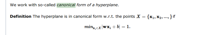
Canonical representation of the decision hyperplanePermalink

source

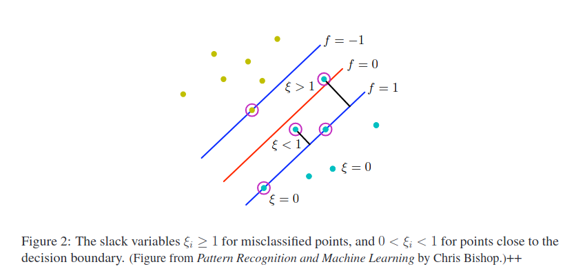
Soft-margin SVMPermalink

• points inside the margin are also support vectors! [source]
• for overlapping class distributions
• still sensitive to outliers because the penalty for misclassification increases linearly with $\xi$
• misclassified points have $\xi_n>1$
• $C$ controls the trade-off between the $\xi_n$ penalty and the margin
• $\sum_n\xi_n$ is an upper bound on the number of misclassified points
  • because $\xi_n>1$
• Note: kernel trick does not avoid curse of dimensionality
  • because any set of points in the original, say, two-dimensional input space $\mathbf{x}$ would be constrained to lie exactly on a two-dimensional nonlinear manifold (depending on the kernel) embedded in the higher-dimensional feature space
    • Note: there are elliptic and hyperbolic paraboloids
• Note: choose monotonically decreasing error function (if the objective is to minimize the misclassification rate)

Limitations of SVMsPermalink

• do not provide posterior probabilistic outputs
  • in contrast, relevance vector machines (RVM) do
    • RVMs are based on a Bayesian formulation
    • they have typically much sparser solutions than SVMs!

Training/Solving the Quadratic Programming ProblemPermalink

• Training phase (i.e., the determination of the parameters $\mathbf{a}$ and $b$) makes use of the whole data set, as opposed to the test phase, which only makes use of the support vectors
  • Problem: Direct solution is often infeasible (demanding computation and memory requirements)
• $\tilde{L}(\mathbf{a})$ is quadratic
  • linear constraints $\Rightarrow$ constraints define a convex region $\Rightarrow$ any local optimum will be a global optimum
• Most popular approach to training SVMs: Sequential minimal optimization (SMO)
  • SMO uses an extreme form of the chunking method
  • standard chunking method:
    • i.e., identifies **all** of the nonzero Lagrange multipliers and discards the others
      • works because Lagrangian does not change, if the rows and columns of the kernel matrix corresponding to Lagrange multipliers that have value zero are removed
        • $\Rightarrow$ size of the matrix in the quadratic function is reduced from $N^2$ to $\left(#(\text{nonzero Lagrange multipliers})\right)^2$, where $N$ is the number of data points
          • Problem: still needs too much memory for large-scale applications
  • SMO considers just **two** Lagrange multipliers at a time, so that the subproblem can be solved analytically instead of numerically
    • those two Lagrange multipliers are chosen using heuristics at each step
  • SMO scaling in practice: between $\mathcal{O}(N)$ and $\mathcal{O}(N^2)$

Probabilistic OutputsPermalink

• SVM does not provide probabilistic outputs
• Platt_2000 has proposed fitting a logistic sigmoid to the outputs of a trained SVM
  • Problem: SVM training process is not geared towards this
    • therefore, the SVM can give poor approximations to the posteriors

AppsPermalink

• Text Classification
  • “Spam or Ham”, spam filter
    • “Bag-of-words” approach
    • Histogram of word counts
      • very high-dimensional feature space ($\approx 10000$ dimensions)
      • few irrelevant features
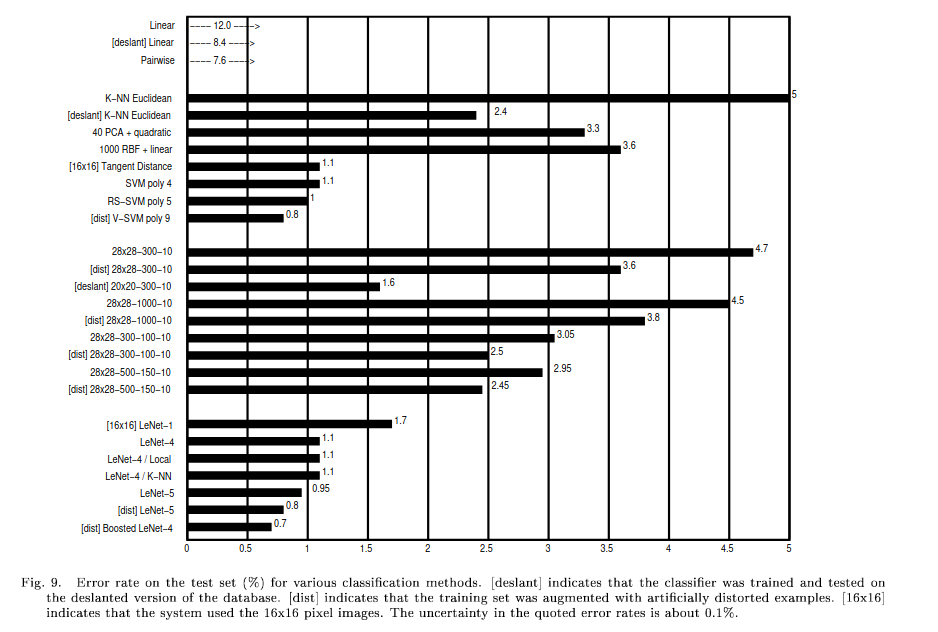
• OCR, Handwritten digit recognition
  • Virtual SVM (V-SVM), Schölkopf, 0.8% error rate on MNIST
    • LeNet-1, 1.7% error rate
    • LeNet-5, 0.95% error rate
  • comparison: overview, see LeNet-5 paper
  • Note: LeNet in general refers to LeNet-5
  • SVMs show **almost no overfitting** with higher-degree kernels!
• Object Detection
  • SVMs are real-time capable
    • sliding-window approach
      • idea: classify “object vs non-object” for each window
        • e.g. pedestrian vs non-pedestrian
• High-energy physics
• protein secondary structure prediction
• etc.

AdaBoostPermalink

• Note: $y_i\in{-1,+1}$ and $h_t\in{-1,+1}$

REFERENCESPermalink

• Bishop, Christopher M., Pattern Recognition and Machine Learning (Information Science and Statistics) (2006), Springer-Verlag, Berlin, Heidelberg, 0387310738.
• Ian J. Goodfellow and Yoshua Bengio and Aaron Courville, Deep Learning (2016), MIT Press, Cambridge, MA, USA