Org
- search
- learn space and time complexities later
- focus on basic properties
Search
- frontier of the search tree: set of unexpanded nodes
- redundant path: a sub-optimal way to get to the same state, e.g. a path containing a cycle
- graph search:
- checks for redundant paths (keeps a table of reached states)
- tree-like search:
- does not check for redundant paths (does not keep a table of reached states)
- branching factor: number of successors of a node that need to be considered
Uninformed Search
Best-first Search
- chooses a node (from the frontier), $n$, with minimum value of some evaluation function, $f(n)$
Breadth-first Search (BFS)
- waves of uniform depth
- best-first search where $f(n)$ is the depth of the node
- complete: always finds a solution with a minimal number of actions (shallowest solution)
- cost-optimal: for problems where all actions have the identical non-negative cost
- time and space complexity: $\mathcal{O}(b^{d+1})$ (with “late goal test”), $\mathcal{O}(b^{d})$ (with “early goal test”)
- The memory requirements are a bigger problem than time
Uniform Cost Search, Dijkstra’s Algorithm, Cheapest-first Search
- waves of uniform path-cost
- best-first search where $f(n)$ is the path-cost of the node
- recall Figure 3.10 example: tests for goals only when it expands a node, not when it generates a node
- always finds cheapest solution, if non-negative action cost for all n
- $\mathcal{O}(b^{1 + \lfloor C^\ast/\epsilon \rfloor})$ time and space complexity, $\epsilon$ cost of cheapest action, $C^\ast$ cost of the cheapest solution
- This is the worst-case time and space complexity: $C^\ast$ is the cost of the optimal solution, $\epsilon$ is a lower bound on the cost of each action, with $\epsilon > 0$. When all action costs are equal $C^\ast / \epsilon = d$, i.e. uniform cost search is similar to BFS.
- Uniform-cost search is complete and is cost-optimal, if non-negative action cost for all n
Depth-first Search
- expands the deepest node in the frontier first
- usually implemented as a tree-like search (s.o.)
- space: $\mathcal{O}(b \cdot m)$, where $m$: max depth
- time: $\mathcal{O}(b^m)$
- not cost-optimal; it returns the first solution it finds, even if it is not cheapest
- complete: when the state space is finite or, more generally, when the diameter of the state space (the maximal distance between any two states reachable by actions) is finite.
- incomplete: can get stuck going down an infinite path ($m=\infty$), even if there are no cycles
- then why use it?
- much smaller needs for memory than BFS
- reason why adopted as the basic workhorse of many areas of AI
Depth-limited Search
- to keep depth-first search from wandering down an infinite path
- depth-first search in which we supply a depth limit, $l$, and treat all nodes at depth $l$ as if they had no successors
- space: $\mathcal{O}(bl)$
- time: $\mathcal{O}(b^l)$
- incomplete: if we make a poor choice for $l$ the algorithm will fail to reach the solution, making it incomplete again
- not cost-optimal; it returns the first solution it finds, even if it is not cheapest (like depth-first search)
- how to find a good depth limit?
- diameter of the state-space graph
- e.g. any city can be reached from any other city in at most 9 actions
- use it as a better depth limit, which leads to a more efficient depth-limited search
- however, for most problems we will not know a good depth limit until we have solved the problem
- diameter of the state-space graph
Iterative Deepening Search
- combines depth-first search and BFS
- solves the problem of picking a good value for $l$ by trying all values: first 0, then 1, then 2, and so on - until either a solution is found, or the depth-limited search returns the
failurevalue rather than thecutoffvalue - space: $\mathcal{O}(bd)$ (better than BFS)
- time: $\mathcal{O}(b^d)$, when there is a solution (asymptotically the same as BFS)
- cost-optimal: for problems where all actions have the identical non-negative cost (like BFS)
- complete, on any finite acyclic state space (like BFS)
- trade-off: breadth-first stores all nodes in memory, while iterative deepening repeats the previous levels, thereby saving memory at the cost of more time
- wasteful because states near the top of the search tree are re-generated multiple times?
- No, because for many state spaces, most of the nodes are in the bottom level, so it does not matter much that the upper levels are repeated
- preferred method when
- the search state space is larger than can fit in memory and
- the depth of the solution is not known
- lecture: iterative deepening is better than BFS (not because of time, but because of space!)
Bidirectional Search
- Assuming that forward and backward search are symmetric
- time: $\mathcal{O}(b^{d/2})$ ideally
- problems:
- Operators not always reversible
- Sometimes there are very many goal states, e.g. chess
- from which one should we start the backward search?
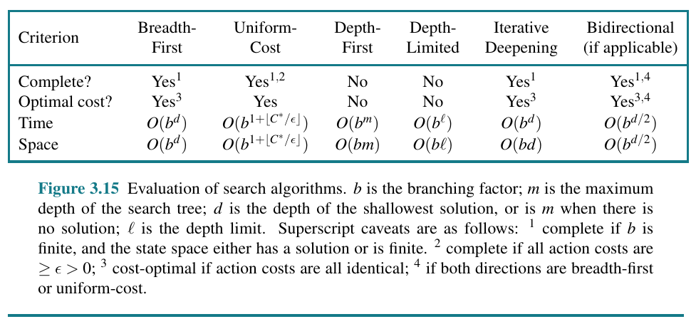
Comparison
Informed Search / Heuristic Search
Greedy Best-first Search
- evaluation function $f(n)=h(n)$ (like $A^\ast$ without $g(n)$)
- complete in finite state spaces, but not in infinite ones
- time and space (worst-case): $\mathcal{O}(\lvert V \rvert)$ ideally, where $V$ is the number of vertices
$A^\ast$ Search
- evaluation function $f(n)=g(n) + h(n)$
- $f(n)$: cost of the full path
- $g(n)$: cost from the initial state to node n
- $h(n)$: estimated cost from node n to a goal state
- an admissible heuristic is one that never overestimates the cost to reach a goal
- $h$ must be admissible for $A^\ast$
- complete, on any finite acyclic state space
- cost-optimal if the heuristic is admissible
- with an inadmissible heuristic $A^\ast$ may or may not be cost-optimal
$\text{IDA}^\ast$ Search
- the cutoff value is the smallest f-cost of any node that exceeded the cutoff on the previous iteration
- see example
Local Search
Hill-climbing Search, Greedy Local Search
- keeps track of one current state
- steepest ascent: on each iteration moves to the neighboring state with highest value
- difficulties:
- Local maxima: can get stuck in local maxima
- Ridges: sequence of local maxima that is very difficult for greedy algorithms to navigate
- Plateaus: can get lost wandering on the plateau
- incomplete: success depends on the shape of the state-space landscape (see point “difficulties”)
- not optimal: solution may not be the best solution (global maximum), but rather a local maximum
- random-restart hill climbing:
- series of hill-climbing searches from randomly generated initial states, until a goal is found
- incomplete: but complete with probability 1, because it will likely eventually generate a goal state as the initial state given enough restarts (but success is still not guaranteed!)
Simulated Annealing
- start by shaking hard (i.e., at a high temperature) and then gradually reduce the intensity of the shaking (i.e., lower the temperature)
- similar to hill climbing, but instead of picking the best move, it picks a random move.
- If the move improves the situation, it is always accepted.
- Otherwise, the algorithm accepts the move with some probability less than 1
- this probability is proportional to the Boltzmann distribution:
-
- E dependence: probability decreases exponentially with the badness of the move, i.e. the amount $\Delta E$ by which the evaluation is worsened,
-
- T dependence: bad moves are more likely to be allowed at the start when T is high, and they become more unlikely as T decreases)
-
- this probability is proportional to the Boltzmann distribution:
Games
Minimax Search
- minimax value: the utility (for MAX) of being in that state (assuming that both players play optimally from there to the end of the game)
- How to determine the minimax value of a state?
- The minimax value of a
- terminal state is just its utility
- non-terminal state,
- MAX prefers to move to a state of maximum value when it is MAX’s turn to move, and
- MIN prefers a state of minimum value
- The minimax value of a
- a Depth-first Search
- therefore, the time and space complexities are the same as for DFS
- space: $\mathcal{O}(b \cdot m)$, where $m$: max depth
- time: $\mathcal{O}(b^m)$
- evaluation function:
- must be easy to compute
- must accurately reflect the probability of winning
- if there are multiple paths with the same evaluation function value, then the evaluation function reflects the probability of winning averaged over all positions with the same evaluation function value
- usually a weighted linear functions (assumes that the criteria are independent of each other!)
- e.g. in chess: “material advantage”: f1=number of white knights, w1=3, f2=number of white pawns, … etc.
- quiescent state:
- those which do not lead to dramatic subsequent changes
- when to CUT OFF search?
- if the state is not quiescent, the evaluation function is misleading → Must not CUT OFF search here! Must look ahead further!
- e.g. in chess: “material advantage” can be misleading
- problem: it is not always possible to look ahead further
- e.g. in chess: “Horizon problem” (delay tactics)
- if the state is not quiescent, the evaluation function is misleading → Must not CUT OFF search here! Must look ahead further!
Suboptimal opponent
- if MIN does not play optimally, then MAX will do at least as well as against an optimal player, possibly better
Alpha-Beta Search
- watch lecture
- see book
- Minimax Search with Alpha-Beta Pruning
- effectiveness (time and space complexity) depends on the ordering of the nodes
- if leaf nodes are random: $\mathcal{O}((b/\log{b})^m)$ for $b>1000$ ($b>1000$ does not apply for most games!)
- try to first examine the successors that are likely to be best: best case time: $\mathcal{O}(b^{m/2})$ (i.e. compared to Minimax Search: effective branching factor $\sqrt{b}$ instead of $b$)
- in practice: With random move ordering: $\mathcal{O}(b^{3m/4})$ for moderate $b$
Expectiminimax
- watch lecture
- see book
- chance nodes (compute the expected value)
- terminal nodes (work the same way as before in Minimax Search)
- MIN and MAX nodes (work the same way as before in Minimax Search)
Knowledge Representation
Definitions
Bound Variable: e.g. the variable is bound by an existential quantifier
Free Variable: if the variable is not bound
Sentence: wff without free variables
Knowledge Base: a set of sentences.
- closed world assumption: the only sentences that are true are those that are entailed by the knowledge base
Sound aka Truth-preserving: An inference algorithm that derives only entailed sentences. An unsound inference procedure essentially makes things up as it goes along. E.g. model checking is sound (if the space of models is finite).
Complete: an inference algorithm is complete if it can derive any sentence that is entailed
Logical Reasoning: inference is performed in the representation space (on “syntax”), but it must correspond to the real world space aspects, i.e. what we infer in the representation space must also make sense in the real world space (see Fig. 7.6)
- “if KB is true in the real world, then any sentence alpha derived from KB by a sound inference procedure is also true in the real world”
- in fact, the conclusions in the representation space must be true in any world in which the premises are true
Grounding: how do we know that KB is true in the real world? E.g. truth of percept sentences like “there is a smell in [1,2]”.
- philosophical question
- the agent’s sensors define if a percept sentence is true
- “the meaning and truth of percept sentences are defined by the processes of sensing and sentence construction that produce them”
Propositional Logic
semantics: rules for determining the truth of a sentence with respect to a particular model
- In propositional logic, truth values are computed recursively.
syntax: the structure of allowable sentences
propositional logic: defines the syntax and the semantics
- In propositional logic, a model simply sets the truth value - true or false - for every proposition symbol
model: assignment of a fixed truth value (true or false) for every propositional symbol
- m satisfies alpha or m is a model of alpha: if a sentence alpha is true in model m (lowercase m)
- notation: M(alpha) = set of all models of alpha
- With $N$ proposition symbols, there are $2^N$ possible models
atomic sentences: single propositional symbol
complex sentences: constructed from simpler sentences, using parentheses and operators called logical connectives
logical connectives: not, and, or, implies, iff
implication or rule or if-then statement
- premise or antecedent
- conclusion or consequent
- propositional logic does not require any relation of causation or relevance between P and Q
- e.g. “5 is odd implies Tokyo is the capital of Japan” is
truein propositional logic
- e.g. “5 is odd implies Tokyo is the capital of Japan” is
- any implication is
truewhenever its antecedent isfalse- e.g. “5 is even implies Sam is smart” is
true
- e.g. “5 is even implies Sam is smart” is
- an implication is
falseonly if P istruebut Q isfalse
iff or biconditional
Model checking
- enumerating all possible models and showing that the sentence $\alpha$ must hold in all models in which KB is
true(Figure 7.5) - in short: $M(KB) \subseteq M(\alpha)$ iff $KB \vDash \alpha$
Theorem Proving
- applying rules of inference directly to the sentences in our knowledge base to construct a proof of the desired sentence without consulting models
- more efficient than model checking, if the number of models is large but the length of the proof is short
Logical Equivalence
- two sentences $\alpha$ and $\beta$ are logically equivalent if they are true in the same set of models
- $\alpha \equiv \beta$ iff $\alpha \vDash \beta$ and $\beta \vDash \alpha$
Validity
- A sentence is valid if it is true in all models
- valid sentence = tautology
- every valid sentence is logically equivalent to True
Deduction Theorem (logical basis for the “Theorem Proving” method)
- $\alpha \vDash \beta$ iff $\alpha \Rightarrow \beta$
- i.e. we can show $\alpha \vDash \beta$ by proving that $(\alpha \Rightarrow \beta)$ is equivalent to
true
- i.e. we can show $\alpha \vDash \beta$ by proving that $(\alpha \Rightarrow \beta)$ is equivalent to
Satisfiability (in propositional logic!)
- A sentence is satisfiable if it is
truein, or satisfied by, some model - can be checked by enumerating the possible models until one is found that satisfies the sentence (SAT problem, NP-complete)
- NP-complete problem: Although a solution to an NP-complete problem can be verified “quickly” (in polynomial time), there is no known way to find a solution quickly (all known algorithms need exponential time).
- $\alpha$ is satisfiable iff $\neg \alpha$ is not valid
- $\alpha$ is valid iff $\neg \alpha$ is unsatisfiable
- For propositional formulae, satisfiability is decidable
- For FOL, satisfiability is undecidable. Furthermore, satisfiability is not semi-decidable.
Proof by contradiction aka Reductio ad absurdum (mathematics)
- $\alpha \vDash \beta$ iff $(\alpha \land \neg \beta)$ is unsatisfiable
- in words: there is no model in which $\alpha$ is true and the negation of $\beta$ is true
Inference Rules:
- Modus Ponens
- And-Elimination
- commutativity of and
- commutativity of or
- associativity of and
- associativity of or
- double-negation elimination
- contraposition
- implication elimination
- biconditional elimination
- De Morgan and
- De Morgan or
- distributivity of and over or
- distributivity of or over and
- resolution
- special case: unit resolution (“unit” refers to “unit clause” = a disjunction of one literal → “ein OR ohne OR”)
Proof can be seen as search problem (see section Search)
- the ACTIONS are all the inference rules applied to all the sentences that match the top half of the inference rule
- more efficient than truth-table algorithm (Fig. 7.10) because the proof can ignore irrelevant propositions, whereas the simple truth-table algorithm, on the other hand, would be overwhelmed by the exponential explosion of models
monotonicity: the set of entailed sentences can only increase as sentences are added to the knowledge base
- $(\text{KB} \vDash \alpha) \Rightarrow (\text{KB}\land\beta \vDash \alpha)$
- i.e. an additional sentence $\beta$ cannot invalidate any conclusion $\alpha$ that was already inferred
Resolution
- an inference rule (like the ones above)
- complementary literals: one is the negation of the other
- clause: disjunction of literals
- unit clause: disjunction of one literal
- takes two clauses and produces a new clause containing all the literals of the two original clauses except the two complementary literals
- resolve only one pair of complementary literals at a time
- the resulting clause should contain only one copy of each literal
- factoring: removal of multiple copies of literals
- yields a complete inference algorithm when coupled with any complete search algorithm (e.g. BFS)
- A resolution-based theorem prover can, for any sentences $\alpha$ and $\beta$ in propositional logic, decide whether $\alpha \vDash \beta$.
- every sentence of propositional logic is logically equivalent to a conjunction of clauses
- CNF or conjunctive normal form: a sentence expressed as a conjunction of clauses is “in CNF”
Resolution Algorithm
- $(\text{KB} \land \neg\alpha)$ is converted into CNF
- the resolution rule is applied to the resulting clauses
- Each pair that contains complementary literals is resolved to produce a new clause, which is added to the set if it is not already present.
- The process continues until one of two things happens
- no new clauses: $\text{KB}$ does not entail $\alpha$
- empty clause: $\text{KB}$ entails $\alpha$
- Note: The empty clause is equivalent to
falsebecause a disjunction istrueonly if at least one of its disjuncts istrue. This is why the resolution algorithm is a proof by contradiction. - Resolution is complete when restricted to MGUs.
- time: exponential $\mathcal{O}(2^n)$ (in the worst case), where $n$ is the number of clauses
- no polynomial time algorithm found yet (but it is not proven that such an algorithm does not exist)
More efficient inference algorithm:
- definite clause: disjunction of literals of which exactly one is positive
- Horn clause: disjunction of literals of which at most one is positive (→ all definite clauses are Horn clauses)
- Horn clauses are closed under resolution
- Deciding entailment with Horn clauses can be done in time that is linear in the size of the knowledge base.
- Inference with Horn clauses can be done through the forward-chaining and backward-chaining algorithms
- easy for humans to follow
- e.g. basis for logic programming
- goal clause: clauses with no positive literals
- k-CNF sentence: CNF sentence where each clause has at most k literals
FOL
- unlike in propositional logic, models in FOL have objects in them
- domain of a model: the set of objects or domain elements it contains
- required to be nonempty, i.e. every possible world must contain at least one object
- object (e.g. “Richard the Lionheart”, “King John”, “left leg of Richard”, “left leg of John”, “crown”)
- relation: the set of tuples of objects that are related
- Note: a tuple is arranged in a fixed order
- binary relation (e.g. “brotherhood”)
- unary relation or property (e.g. “person”, “king”, “crown”)
- function: a given object must be related to exactly one object in this way (e.g. the “left leg” function)
- total functions: there must be a value for every input tuple (e.g. every object must have a “left leg”)
- models in FOL require total functions
- Syntax
- all symbols begin with uppercase letters
- constant symbols, which stand for objects (e.g. Richard, John)
- predicate symbols, which stand for relations (e.g. Brother, OnHead, Person, King, and Crown)
- function symbols, which stand for functions (e.g. LeftLeg)
- arity: number of arguments of a function symbol
- symbols stehen für (objects, relations oder functions), aber für welche genau sie stehen muss die interpretation spezifizieren
- model in FOL: consists of
- set of objects
- interpretation: maps constant symbols to objects, function symbols to functions on those objects, and predicate symbols to relations
- Note: not all the objects need have a name
- term: logical expression that refers to an object (e.g. constant symbols, function symbols “LeftLeg(John)”, variables)
- Semantics: Consider a term $f(t_1,\dots,t_n)$:
- The function symbol $f$ refers to some function in the model (call it $F$);
- the argument terms refer to objects in the domain (call them $d1,\dots,dn$);
- the term as a whole refers to the object that is the value of the function $F$ applied to $d_1,\dots,d_n$
- atomic sentences or atoms: predicate symbol optionally followed by a parenthesized list of terms (e.g. Brother(Richard, John))
- An atomic sentence is
truein a given model if the relation referred to by the predicate symbol holds among the objects referred to by the arguments
- An atomic sentence is
- Universal Quantifier: $\forall x \text{King}(x) \Rightarrow \text{Person}(x)$ (“For all x, if x is a king, then x is a person.”)
- $\forall x P$ is
truein a given model if $P$ istruein all extended interpretations that assign $x$ to a domain element
- $\forall x P$ is
- Existential Quantifier:
- $\exists x P$ is
truein a given model if $P$ istruein at least one extended interpretation that assigns $x$ to a domain element
- $\exists x P$ is
- variable
- lowercase letters
- ground term: a term with no variables
- unique names assumption: every constant and every ground term refers to a distinct object
- assertion: a sentence added to a KB by using
TELL - query or goal: a question asked with
ASK- Generally speaking, any query that is logically entailed by the knowledge base should be answered with
true
- Generally speaking, any query that is logically entailed by the knowledge base should be answered with
- ASKVARS: yields a stream of answers, i.e. a substitution list or binding list
- useful e.g. for the query $\text{ASK}(\text{KB}, \exists x \text{ Person}(x))$
Inference in FOL
- algorithms that can answer any answerable first-order logic question
Propositional vs First-Order Inference
- ground term: a term without variables
- substitution: e.g. {$x/\text{Father}(\text{John})$} is also a substitution, i.e. substituting with functions is allowed (see 9.1 intro)
- only substitute free variables, not the bound variables!
- Inference rules for quantifiers
- Universal Instantiation rule: we can infer any sentence obtained by substituting a ground term (a term without variables) for a universally quantified variable
- Existential Instantiation rule: replaces an existentially quantified variable with a single new constant symbol (aka Skolem constant)
- the new constant symbol must not already belong to another object
- propositionalization: reduce first-order inference to propositional inference
- apply UI using all possible substitutions
- replace ground atomic sentences, such as King(John), with proposition symbols, such as JohnIsKing
- apply any of the complete propositional algorithms to obtain conclusions such as JohnIsEvil, which is equivalent to Evil(John)
- problem with propositionalization: when the knowledge base includes a function symbol, the set of possible ground-term substitutions is infinite
- Herbrand’s Theorem: If a sentence is entailed by the original, first-order KB, then there is a proof involving just a finite subset of the propositionalized knowledge base.
- We can find this subset!
- propositionalization is complete: any entailed sentence can be proved (using propositionalization)
- But: we cannot tell if the sentence is entailed or not in the first place (in FOL entailment is semidecidable)
- i.e. the proof procedure can go on and on but we will not know whether it is stuck in a loop or whether the proof is just about to pop out
- But: we cannot tell if the sentence is entailed or not in the first place (in FOL entailment is semidecidable)
Unification
- inference rules that work directly with first-order sentences
Resolution-based Theorem Proving
- Every sentence of first-order logic can be converted into an inferentially equivalent CNF sentence.
CNF for FOL
- Eliminate implications
- Move $\lnot$ inwards
- Standardize variables
- Skolemize
- Drop universal quantifiers
- Distribute $\lor$ over $\land$
- Apply resolution: first-order literals are complementary if one unifies with the negation of the other
- factoring:
- i.e. removal of redundant literals
- first-order factoring reduces two literals to one if they are unifiable.
- The unifier must be applied to the entire clause
Herbrand’s Theorem
Herbrand universe: If $S$ is a set of clauses, then $H_S$, is the set of all ground terms constructible from
- the function symbols in $S$
- the constant symbols in $S$ Saturation $P(S)$: the set of all ground clauses obtained by applying all possible consistent substitutions of ground terms in $P$ for variables in $S$ Herbrand Base: the saturation of a set $S$ of clauses with respect to its Herbrand universe
Herbrand’s Theorem: If a set $S$ of clauses is unsatisfiable, then there exists a finite subset of $H_S(S)$ that is also unsatisfiable.
- Lakemeyer lecture: $S$ is satisfiable iff the Herbrand base is satisfiable
Logic Programming, Prolog
- Prolog is the most widely used logic programming language.
- It is used primarily
- as a rapid-prototyping language and
- for symbol-manipulation tasks such as
- writing compilers (Van Roy, 1990) and
- parsing natural language (Pereira and Warren, 1980).
- Many expert systems have been written in Prolog for legal, medical, financial, and other domains
- for constraint satisfaction / constraint programming:
- The first language created expressly with intrinsic support for constraint programming was Prolog.