PyTorch 101, Part 1: Understanding Graphs, Automatic Differentiation and Autograd
In this article, we dive into how PyTorch’s Autograd engine performs automatic differentiation.
3 years ago • 13 min read
MathJax.Hub.Config({ tex2jax: { inlineMath: [[”$”, “$”], [”\(”, “\)”]], processEscapes: true } });
PyTorch is one of the foremost python deep learning libraries out there. It’s the go to choice for deep learning research, and as each days passes by, more and more companies and research labs are adopting this library.
In this series of tutorials, we will be introducing you to PyTorch, and how to make the best use of the libraries as well the ecosystem of tools built around it. We’ll first cover the basic building blocks, and then move onto how you can quickly prototype custom architectures. We will finally conclude with a couple of posts on how to scale your code, and how to debug your code if things go awry.
This is Part 1 of our PyTorch 101 series.
- Understanding Graphs, Automatic Differentiation and Autograd
- Building Your First Neural Network
- Going Deep with PyTorch
- Memory Management and Using Multiple GPUs
- Understanding Hooks
You can get all the code in this post, (and other posts as well) in the Github repo here.
Prerequisites
- Chain rule
- Basic Understanding of Deep Learning
- PyTorch 1.0
You can get all the code in this post, (and other posts as well) in the Github repo here.
Automatic Differentiation
A lot of tutorial series on PyTorch would start begin with a rudimentary discussion of what the basic structures are. However, I’d like to instead start by discussing automatic differentiation first.
Automatic Differentiation is a building block of not only PyTorch, but every DL library out there. In my opinion, PyTorch’s automatic differentiation engine, called Autograd is a brilliant tool to understand how automatic differentiation works. This will not only help you understand PyTorch better, but also other DL libraries.
Modern neural network architectures can have millions of learnable parameters. From a computational point of view, training a neural network consists of two phases:
- A forward pass to compute the value of the loss function.
- A backward pass to compute the gradients of the learnable parameters.
The forward pass is pretty straight forward. The output of one layer is the input to the next and so forth.
Backward pass is a bit more complicated since it requires us to use the chain rule to compute the gradients of weights w.r.t to the loss function.
A toy example
Let us take an very simple neural network consisting of just 5 neurons. Our neural network looks like the following.
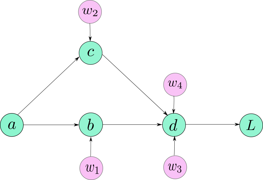
A Very Simple Neural Network
The following equations describe our neural network.
\(b = w\_1 * a\) \(c = w\_2 * a\) \(d = w\_3 * b + w\_4 * c\) \(L = 10 - d\)
Let us compute the gradients for each of the learnable parameters $w$.
\(\\frac{\\partial{L}}{\\partial{w\_4}} = \\frac{\\partial{L}}{\\partial{d}} * \\frac{\\partial{d}}{\\partial{w\_4}}\) \(\\frac{\\partial{L}}{\\partial{w\_3}} = \\frac{\\partial{L}}{\\partial{d}} * \\frac{\\partial{d}}{\\partial{w\_3}}\) \(\\frac{\\partial{L}}{\\partial{w\_2}} = \\frac{\\partial{L}}{\\partial{d}} * \\frac{\\partial{d}}{\\partial{c}} * \\frac{\\partial{c}}{\\partial{w\_2}}\) \(\\frac{\\partial{L}}{\\partial{w\_1}} = \\frac{\\partial{L}}{\\partial{d}} * \\frac{\\partial{d}}{\\partial{b}} * \\frac{\\partial{b}}{\\partial{w\_1}}\)
All these gradients have been computed by applying the chain rule. Note that all the individual gradients on the right hand side of the equations mentioned above can be computed directly since the numerators of the gradients are explicit functions of the denominators.
Computation Graphs
We could manually compute the gradients of our network as it was very simple. Imagine, what if you had a network with 152 layers. Or, if the network had multiple branches.
When we design software to implement neural networks, we want to come up with a way that can allow us to seamlessly compute the gradients, regardless of the architecture type so that the programmer doesn’t have to manually compute gradients when changes are made to the network.
We galvanise this idea in form of a data structure called a Computation graph. A computation graph looks very similar to the diagram of the graph that we made in the image above. However, the nodes in a computation graph are basically operators. These operators are basically the mathematical operators except for one case, where we need to represent creation of a user-defined variable.
Notice that we have also denoted the leaf variables $ a, w_1, w_2, w_3, w_4$ in the graph for sake of clarity. However, it should noted that they are not a part of the computation graph. What they represent in our graph is the special case for user-defined variables which we just covered as an exception.

Computation Graph for our very simple Neural Network
The variables, b,c and d are created as a result of mathematical operations, whereas variables a, w1, w2, w3 and w4 are initialised by the user itself. Since, they are not created by any mathematical operator, nodes corresponding to their creation is represented by their name itself. This is true for all the leaf nodes in the graph.
Computing the gradients
Now, we are ready to describe how we will compute gradients using a computation graph.
Each node of the computation graph, with the exception of leaf nodes, can be considered as a function which takes some inputs and produces an output. Consider the node of the graph which produces variable d from $ w_4c$ and $w_3b$. Therefore we can write,
\[d = f(w\_3b , w\_4c)\]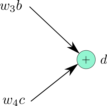
d is output of function f(x,y) = x + y
Now, we can easily compute the gradient of the $f$ with respect to it’s inputs, $\frac{\partial{f}}{\partial{w_3b}}$ and $\frac{\partial{f}}{\partial{w_4c}}$ (which are both 1). Now, label the edges coming into the nodes with their respective gradients like the following image.
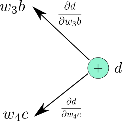
Local Gradients
We do it for the entire graph. The graph looks like this.
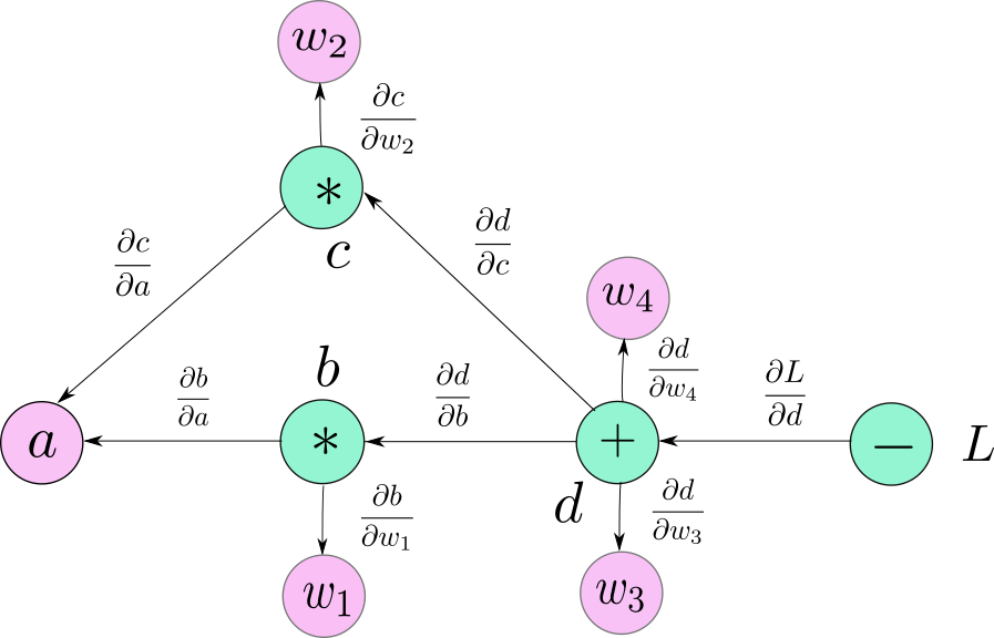
Backpropagation in a Computational Graph
Following we describe the algorithm for computing derivative of any node in this graph with respect to the loss, $L$. Let’s say we want to compute the derivative, $\frac{\partial{f}}{\partial{w_4}}$.
- We first trace down all possible paths from d to $ w_4 $.
- There is only one such path.
- We multiply all the edges along this path.
If you see, the product is precisely the same expression we derived using chain rule. If there is more than one path to a variable from L then, we multiply the edges along each path and then add them together. For example, $\frac{\partial{L}}{\partial{a}}$ is computed as
\[\\frac{\\partial{f}}{\\partial{w_4}} = \\frac{\\partial{L}}{\\partial{d}}*\\frac{\\partial{d}}{\\partial{b}}*\\frac{\\partial{b}}{\\partial{a}} + \\frac{\\partial{L}}{\\partial{d}}*\\frac{\\partial{d}}{\\partial{c}}*\\frac{\\partial{c}}{\\partial{a}}\]PyTorch Autograd
Now we get what a computational graph is, let’s get back to PyTorch and understand how the above is implemented in PyTorch.
Tensor
Tensor is a data structure which is a fundamental building block of PyTorch. Tensors are pretty much like numpy arrays, except that unlike numpy, tensors are designed to take advantage of parallel computation capabilities of a GPU. A lot of Tensor syntax is similar to that of numpy arrays.
In [1]:  import torch

In [2]: tsr = torch.Tensor(3,5)

In [3]: tsr
Out[3]:
tensor([[ 0.0000e+00,  0.0000e+00,  8.4452e-29, -1.0842e-19,  1.2413e-35],
        [ 1.4013e-45,  1.2416e-35,  1.4013e-45,  2.3331e-35,  1.4013e-45],
        [ 1.0108e-36,  1.4013e-45,  8.3641e-37,  1.4013e-45,  1.0040e-36]])
One it’s own, Tensor is just like a numpy ndarray. A data structure that can let you do fast linear algebra options. If you want PyTorch to create a graph corresponding to these operations, you will have to set the requires_grad attribute of the Tensor to True.
The API can be a bit confusing here. There are multiple ways to initialise tensors in PyTorch. While some ways can let you explicitly define that the requires_grad in the constructor itself, others require you to set it manually after creation of the Tensor.
>> t1 = torch.randn((3,3), requires_grad = True)

>> t2 = torch.FloatTensor(3,3) # No way to specify requires_grad while initiating
>> t2.requires_grad = True
requires_grad is contagious. It means that when a Tensor is created by operating on other Tensors, the requires_grad of the resultant Tensor would be set True given at least one of the tensors used for creation has it’s requires_grad set to True.
Each Tensor has a something an attribute called grad_fn, which refers to the mathematical operator that create the variable. If requires_grad is set to False, grad_fn would be None.
In our example where, $ d = f(w_3b , w_4c) $, d’s grad function would be the addition operator, since f adds it’s to input together. Notice, addition operator is also the node in our graph that output’s d. If our Tensor is a leaf node (initialised by the user), then the grad_fn is also None.
import torch

a = torch.randn((3,3), requires_grad = True)

w1 = torch.randn((3,3), requires_grad = True)
w2 = torch.randn((3,3), requires_grad = True)
w3 = torch.randn((3,3), requires_grad = True)
w4 = torch.randn((3,3), requires_grad = True)

b = w1*a
c = w2*a

d = w3*b + w4*c

L = 10 - d

print("The grad fn for a is", a.grad_fn)
print("The grad fn for d is", d.grad_fn)
If you run the code above, you get the following output.
The grad fn for a is None
The grad fn for d is <AddBackward0 object at 0x1033afe48>
One can use the member function is_leaf to determine whether a variable is a leaf Tensor or not.
Function
All mathematical operations in PyTorch are implemented by the torch.nn.Autograd.Function class. This class has two important member functions we need to look at.
The first is it’s forward function, which simply computes the output using it’s inputs.
The backward function takes the incoming gradient coming from the the part of the network in front of it. As you can see, the gradient to be backpropagated from a function f is basically the gradient that is backpropagated to f from the layers in front of it multiplied by the local gradient of the output of f with respect to it’s inputs. This is exactly what the backward function does.
Let’s again understand with our example of \(d = f(w\_3b , w\_4c)\)
- d is our
Tensorhere. It’sgrad_fnis<ThAddBackward>. This is basically the addition operation since the function that creates d adds inputs. - The
forwardfunction of the it’sgrad_fnreceives the inputs $w_3b$ and $w_4c$ and adds them. This value is basically stored in the d - The
backwardfunction of the<ThAddBackward>basically takes the the incoming gradient from the further layers as the input. This is basically $\frac{\partial{L}}{\partial{d}}$ coming along the edge leading from L to d. This gradient is also the gradient of L w.r.t to d and is stored ingradattribute of thed. It can be accessed by callingd.grad. - It then takes computes the local gradients $\frac{\partial{d}}{\partial{w_4c}}$ and $\frac{\partial{d}}{\partial{w_3b}}$.
- Then the backward function multiplies the incoming gradient with the locally computed gradients respectively and “_sends“_ the gradients to it’s inputs by invoking the backward method of the
grad_fnof their inputs. - For example, the
backwardfunction of<ThAddBackward>associated with d invokes backward function of the grad_fn of the $w_4*c$ (Here, $w_4*c$ is a intermediate Tensor, and it’s grad_fn is<ThMulBackward>. At time of invocation of thebackwardfunction, the gradient $\frac{\partial{L}}{\partial{d}} * \frac{\partial{d}}{\partial{w_4c}} $ is passed as the input. - Now, for the variable $w_4*c$, $\frac{\partial{L}}{\partial{d}} * \frac{\partial{d}}{\partial{w_4c}} $ becomes the incoming gradient, like $\frac{\partial{L}}{\partial{d}} $ was for $_d$_ in step 3 and the process repeats.
Algorithmically, here’s how backpropagation happens with a computation graph. (Not the actual implementation, only representative)
def backward (incoming_gradients):
	self.Tensor.grad = incoming_gradients

	for inp in self.inputs:
		if inp.grad_fn is not None:
			new_incoming_gradients = //
			  incoming_gradient * local_grad(self.Tensor, inp)

			inp.grad_fn.backward(new_incoming_gradients)
		else:
			pass
Here, self.Tensor is basically the Tensor created by Autograd.Function, which was d in our example.
Incoming gradients and local gradients have been described above.
In order to compute derivatives in our neural network, we generally call backward on the Tensor representing our loss. Then, we backtrack through the graph starting from node representing the grad_fn of our loss.
As described above, the backward function is recursively called through out the graph as we backtrack. Once, we reach a leaf node, since the grad_fn is None, but stop backtracking through that path.
One thing to note here is that PyTorch gives an error if you call backward() on vector-valued Tensor. This means you can only call backward on a scalar valued Tensor. In our example, if we assume a to be a vector valued Tensor, and call backward on L, it will throw up an error.
import torch

a = torch.randn((3,3), requires_grad = True)

w1 = torch.randn((3,3), requires_grad = True)
w2 = torch.randn((3,3), requires_grad = True)
w3 = torch.randn((3,3), requires_grad = True)
w4 = torch.randn((3,3), requires_grad = True)

b = w1*a
c = w2*a

d = w3*b + w4*c

L = (10 - d)

L.backward()
Running the above snippet results in the following error.
RuntimeError: grad can be implicitly created only for scalar outputs
This is because gradients can be computed with respect to scalar values by definition. You can’t exactly differentiate a vector with respect to another vector. The mathematical entity used for such cases is called a Jacobian, the discussion of which is beyond the scope of this article.
There are two ways to overcome this.
If you just make a small change in the above code setting L to be the sum of all the errors, our problem will be solved.
import torch

a = torch.randn((3,3), requires_grad = True)

w1 = torch.randn((3,3), requires_grad = True)
w2 = torch.randn((3,3), requires_grad = True)
w3 = torch.randn((3,3), requires_grad = True)
w4 = torch.randn((3,3), requires_grad = True)

b = w1*a
c = w2*a

d = w3*b + w4*c

# Replace L = (10 - d) by
L = (10 -d).sum()

L.backward()
Once that’s done, you can access the gradients by calling the grad attribute of Tensor.
Second way is, for some reason have to absolutely call backward on a vector function, you can pass a torch.ones of size of shape of the tensor you are trying to call backward with.
# Replace L.backward() with
L.backward(torch.ones(L.shape))
Notice how backward used to take incoming gradients as it’s input. Doing the above makes the backward think that incoming gradient are just Tensor of ones of same size as L, and it’s able to backpropagate.
In this way, we can have gradients for every Tensor , and we can update them using Optimisation algorithm of our choice.
w1 = w1 - learning_rate * w1.grad
And so on.
How are PyTorch’s graphs different from TensorFlow graphs
PyTorch
PyTorch creates something called a Dynamic Computation Graph, which means that the graph is generated on the fly.
Until the forward function of a Variable is called, there exists no node for the Tensor (it’s grad_fn) in the graph.
    a = torch.randn((3,3), requires_grad = True)   #No graph yet, as a is a leaf

    w1 = torch.randn((3,3), requires_grad = True)  #Same logic as above

    b = w1*a   #Graph with node `mulBackward` is created.
The graph is created as a result of forward function of many Tensors being invoked. Only then, the buffers for the non-leaf nodes are allocated for the graph and intermediate values (used for computing gradients later). When you call backward, as the gradients are computed, these buffers (for non-leaf variables) are essentially freed, and the graph is destroyed (In a sense, you can't backpropagate through it, since the buffers holding values to compute the gradients are gone).
Next time, you will call forward on the same set of tensors, the leaf node buffers from the previous run will be shared, while the non-leaf nodes buffers will be created again.
If you call backward more than once on a graph with non-leaf nodes, you'll be met with the following error.
RuntimeError: Trying to backward through the graph a second time, but the buffers have already been freed. Specify retain_graph=True when calling backward the first time.
This is because the non-leaf buffers gets destroyed the first time backward() is called and hence, there’s no path to navigate to the leaves when backward is invoked the second time. You can undo this non-leaf buffer destroying behaviour by adding retain_graph = True argument to the backward function.
loss.backward(retain_graph = True)
If you do the above, you will be able to backpropagate again through the same graph and the gradients will be accumulated, i.e. the next time you backpropagate, the gradients will be added to those already stored in the previous back pass.
TensorFlow
This is in contrast to the Static Computation Graphs, used by TensorFlow where the graph is declared before running the program. Then the graph is “run” by feeding values to the predefined graph.
The dynamic graph paradigm allows you to make changes to your network architecture during runtime, as a graph is created only when a piece of code is run.
This means a graph may be redefined during the lifetime for a program since you don’t have to define it beforehand.
This, however, is not possible with static graphs where graphs are created before running the program, and merely executed later.
Dynamic graphs also make debugging way easier since it’s easier to locate the source of your error.
Some Tricks of Trade
requires_grad
This is an attribute of the Tensor class. By default, it’s False. It comes handy when you have to freeze some layers, and stop them from updating parameters while training. You can simply set the requires_grad to False, and these Tensors won’t participate in the computation graph.
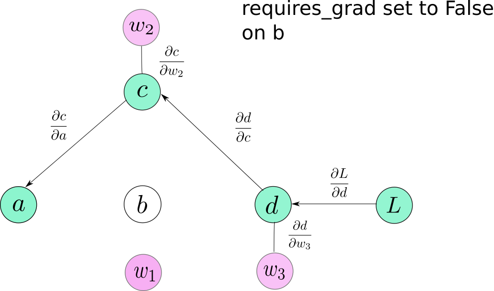
Thus, no gradient would be propagated to them, or to those layers which depend upon these layers for gradient flow requires_grad. When set to True, requires_grad is contagious meaning even if one operand of an operation has requires_grad set to True, so will the result.
torch.no_grad()
When we are computing gradients, we need to cache input values, and intermediate features as they maybe required to compute the gradient later.
The gradient of $ b = w_1*a $ w.r.t it’s inputs $w_1$ and $a$ is $a$ and $w_1$ respectively. We need to store these values for gradient computation during the backward pass. This affects the memory footprint of the network.
While, we are performing inference, we don’t compute gradients, and thus, don’t need to store these values. Infact, no graph needs to be create during inference as it will lead to useless consumption of memory.
PyTorch offers a context manager, called torch.no_grad for this purpose.
with torch.no_grad:
	inference code goes here
No graph is defined for operations executed under this context manager.
Conclusion
Understanding how Autograd and computation graphs works can make life with PyTorch a whole lot easier. With our foundations rock solid, the next posts will detail how to create custom complex architectures, how to create custom data pipelines and more interesting stuff.