Neural Networks
Perceptrons (Rosenblatt 1962)
- perceptrons are generalized linear models (“generalized” because of the activation function)
- BUT: Deep Neural Networks are nonlinear parametric models.
- more specifically: perceptrons are generalized linear discriminants (because they map the input x directly to a class label t in {-1,+1} [see above: “Linear models for classification”: approach 1.])
- original version:
- 2-class linear discriminant
- with fixed [i.e. not learned!] nonlinear transformation $\vec{\phi}(\pmb{x})$
- activation function: step function
- learned via minimization of “perceptron criterion” $\Rightarrow$ SGD
- exact solution guaranteed for linearly separable data set (Perceptron Convergence Theorem)
- BUT: in practice, convergence can be slow
- it’s hard to decide, if a problem is not linearly separable or just slowly converging!
- BUT: in practice, convergence can be slow
Terminology
-
Input layer is a layer, it’s not wrong to say that. source
-
However, when calculating the depth of a deep neural network, we only consider the layers that have tunable weights. source
Automatic Differentiation
Forward-mode vs Reverse-mode differentiation
- read Olah
Forward-mode differentiation starts at an input to the graph and moves towards the end. At every node, it sums all the paths feeding in. Each of those paths represents one way in which the input affects that node. By adding them up, we get the total way in which the node is affected by the input, it’s derivative. […]
Reverse-mode differentiation, on the other hand, starts at an output of the graph and moves towards the beginning. At each node, it merges all paths which originated at that node. […]
When I say that reverse-mode differentiation gives us the derivative of e with respect to every node, I really do mean every node. We get both $\frac{\partial e}{\partial a}$ and $\frac{\partial e}{\partial b}$, the derivatives of $e$ with respect to both inputs. Forward-mode differentiation gave us the derivative of our output with respect to a single input, but reverse-mode differentiation gives us all of them. […]
When training neural networks, we think of the cost (a value describing how bad a neural network performs) as a function of the parameters (numbers describing how the network behaves). We want to calculate the derivatives of the cost with respect to all the parameters, for use in gradient descent. Now, there’s often millions, or even tens of millions of parameters in a neural network. So, reverse-mode differentiation, called backpropagation [more precise: reverse_mode_accumulation] in the context of neural networks, gives us a massive speed up!
(Are there any cases where forward-mode differentiation makes more sense? Yes, there are! Where the reverse-mode gives the derivatives of one output with respect to all inputs, the forward-mode gives us the derivatives of all outputs with respect to one input. If one has a function with lots of outputs, forward-mode differentiation can be much, much, much faster.)
- both are algorithms for efficiently computing the sum by factoring the paths. Instead of summing over all of the paths explicitly, they compute the same sum more efficiently by **merging paths back together at every node**. In fact, both algorithms touch each edge exactly once!
- At each node, reverse-mode differentiation merges all paths which originated at that node (starting at an output of the graph and moving towards the beginning)
- At each node, forward-mode differentiation sums all the paths feeding into that node (starting at the beginning and moving towards an output of the graph)
- forward-mode: apply operator $\frac{\partial}{\partial X}$
- reverse-mode: apply operator $\frac{\partial Z}{\partial}$
- if we have e.g. a hundred inputs, but only one output, reverse-mode differentiation gives a speed up in $\mathcal{O}(\text{# Inputs})$ compared to forward-mode differentiation
PyTorch autograd
- In the above examples, we had to manually implement both the forward and backward passes of our neural network. Manually implementing the backward pass is not a big deal for a small two-layer (?: siehe Stichpunkt) network, but can quickly get very hairy for large complex networks.
- ?: Why “two-layer”:
- The previous polynomial regression examples correspond to a single layer perceptron with a fixed nonlinear transformation of the inputs (here: using polynomial basis functions), so why does Johnson say two-layer perceptron?
- What Johnson probably means here is that, basically, implementing backprop manually (like in the previous polynomial regression examples) for a two-layer NN would be possible without autograd. This “two-layer network”, however, does not refer to the previous polynomial regression models!
- The previous polynomial regression examples correspond to a single layer perceptron with a fixed nonlinear transformation of the inputs (here: using polynomial basis functions), so why does Johnson say two-layer perceptron?
- ?: Why “two-layer”:
autogradcomputes all gradients with only one lineloss.backward().- in polynomial regression example without
autograd:grad_a = grad_y_pred.sum() grad_b = (grad_y_pred * x).sum() grad_c = (grad_y_pred * x ** 2).sum() grad_d = (grad_y_pred * x ** 3).sum() - the same with
autograd:loss.backward()where all parameter tensors must have
requires_grad = True(otherwiseautograddoes not know wrt which parameterslossmust be differentiated).
- in polynomial regression example without
- Thankfully, we can use automatic differentiation to automate the computation of backward passes in neural networks. The autograd package in PyTorch provides exactly this functionality. When using autograd, the forward pass of your network will define a computational graph; nodes in the graph will be Tensors, and edges will be functions that produce output Tensors from input Tensors. Backpropagating through this graph then allows you to easily compute gradients.
- auf Folie:
- Convert NN to a computational graph
- Each new layer/module specifies how it affects the forward and backward passes
- auf nächster Folie: “Each module is defined by
module.fprop($x$)module.bprop($\frac{\partial E}{\partial y}$)- computes the gradients of the cost wrt. the inputs $x$ given the gradient wrt. the outputs $y$
module.bprop()ist in PyTorch wegen dem Autograd System nicht notwendig (vgl. aus PyTorch Doc)
- e.g.
torch.nn.Linearspecifies that it will apply a linear transformation $y=xA^T+b$ to the incoming data during the forward pass (each module has aforward()method, see e.g. source nn.Linear)
- auf nächster Folie: “Each module is defined by
- Apply reverse-mode differentiation
- i.e. call
loss.backward()
- i.e. call
- auf Folie:
- This sounds complicated, it’s pretty simple to use in practice. Each Tensor represents a node in a computational graph. If
xis a Tensor that hasx.requires_grad=Truethenx.gradis another Tensor holding the gradient ofxwith respect to some scalar value.
# -*- coding: utf-8 -*-
import torch
import math


# Create Tensors to hold input and outputs.
x = torch.linspace(-math.pi, math.pi, 2000)
y = torch.sin(x)

# For this example, the output y is a linear function of (x, x^2, x^3), so
# we can consider it as a linear layer neural network. Let's prepare the
# tensor (x, x^2, x^3).
p = torch.tensor([1, 2, 3])
xx = x.unsqueeze(-1).pow(p)

# In the above code, x.unsqueeze(-1) has shape (2000, 1), and p has shape
# (3,), for this case, broadcasting semantics will apply to obtain a tensor
# of shape (2000, 3)

# Use the nn package to define our model as a sequence of layers. nn.Sequential
# is a Module which contains other Modules, and applies them in sequence to
# produce its output. The Linear Module computes output from input using a
# linear function, and holds internal Tensors for its weight and bias.
# The Flatten layer flatens the output of the linear layer to a 1D tensor,
# to match the shape of `y`.
model = torch.nn.Sequential(
    torch.nn.Linear(3, 1),
    torch.nn.Flatten(0, 1)
)

# The nn package also contains definitions of popular loss functions; in this
# case we will use Mean Squared Error (MSE) as our loss function.
loss_fn = torch.nn.MSELoss(reduction='sum')

learning_rate = 1e-6
for t in range(2000):

    # Forward pass: compute predicted y by passing x to the model. Module objects
    # override the __call__ operator so you can call them like functions. When
    # doing so you pass a Tensor of input data to the Module and it produces
    # a Tensor of output data.
    y_pred = model(xx)

    # Compute and print loss. We pass Tensors containing the predicted and true
    # values of y, and the loss function returns a Tensor containing the
    # loss.
    loss = loss_fn(y_pred, y)
    if t % 100 == 99:
        print(t, loss.item())

    # Zero the gradients before running the backward pass.
    model.zero_grad()

    # Backward pass: compute gradient of the loss with respect to all the learnable
    # parameters of the model. Internally, the parameters of each Module are stored
    # in Tensors with requires_grad=True, so this call will compute gradients for
    # all learnable parameters in the model.
    loss.backward()

    # Update the weights using gradient descent. Each parameter is a Tensor, so
    # we can access its gradients like we did before.
    with torch.no_grad():
        for param in model.parameters():
            param -= learning_rate * param.grad

# You can access the first layer of `model` like accessing the first item of a list
linear_layer = model[0]

# For linear layer, its parameters are stored as `weight` and `bias`.
print(f'Result: y = {linear_layer.bias.item()} + {linear_layer.weight[:, 0].item()} x + {linear_layer.weight[:, 1].item()} x^2 + {linear_layer.weight[:, 2].item()} x^3')
Forward Propagation
- inputs:
- depth $l$
- $l$ weight matrices of the model $\mathbf{W}^{(i)}$
- $l$ biases of the model $\mathbf{b}^{(i)}$
- input $\mathbf{x}$ (here: only one for simplicity)
- target $\mathbf{y}$
- outputs:
- output $\hat{\mathbf{y}}$
- cost function $J$
- input of unit $j$: $\mathbf{a}_j^{(k)}$ for all $j$
- output of unit $j$: $\mathbf{h}_j^{(k)}$ for all $j$
Backprop
- inputs:
- depth l
- l weight matrices of the model $\mathbf{W}^{(i)}$
- l biases of the model $\mathbf{b}^{(i)}$
- outputs of Forward Propagation
- outputs:
- gradients w.r.t. all weights and biases $\nabla_{\mathbf{W}^{(k)}}J$ and $\nabla_{\mathbf{b}^{(k)}}J$
- also computes all $\nabla_{\mathbf{a}^{(k)}}J$ and $\nabla_{\mathbf{h}^{(k)}}J$ in the process
- $\nabla_{\mathbf{a}^{(k)}}J$ can be interpreted as an indication of how each layer’s output should change to reduce error
- es gibt ein $\nabla_{\mathbf{a}^{(k)}}J$ pro layer k: jede unit in layer k entspricht einer Komponente von $\nabla_{\mathbf{a}^{(k)}}J$
- $\nabla_{\mathbf{a}^{(k)}}J$ can be interpreted as an indication of how each layer’s output should change to reduce error
- also computes all $\nabla_{\mathbf{a}^{(k)}}J$ and $\nabla_{\mathbf{h}^{(k)}}J$ in the process
- gradients w.r.t. all weights and biases $\nabla_{\mathbf{W}^{(k)}}J$ and $\nabla_{\mathbf{b}^{(k)}}J$
- refers only to the method used to compute all necessary gradients, whereas another algorithm (e.g. SGD) is used to perform learning using these gradients!
- “however, the term is often used loosely to refer to the entire learning algorithm, including how the gradient is used, such as by stochastic gradient descent” source > “More generally, the field of automatic differentiation is concerned with how to compute derivatives algorithmically. The back-propagation algorithm described here is only one approach to automatic differentiation. It is a special case of a broader class of techniques called reverse mode accumulation.” (Goodfellow, Bengio)
- “layer below builds upon (gradient) result of layer above” (basically, chain rule)
- this is why it’s called “backprop”
- “propagates the gradient backwards through the layers”
- “performs on the order of one Jacobian product per node in the graph” (Goodfellow, Bengio)
- This can be seen from the fact that Backprop visits each edge (of the computational graph for this problem) only once
- “[…] the amount of computation required for performing the back-propagation scales linearly with the number of edges in $\mathcal{G}$, where the computation for each edge corresponds to computing
- a partial derivative (of one node with respect to one of its parents) as well as performing
- one multiplication and
- one addition.” (Goodfellow, Bengio)
Computational Graphs
- the following texts from Goodfellow_2016 describe the same graphs as Olah is describing in his blog post
- “That algorithm specifies the forward propagation computation, which we could put in a graph $\mathcal{G}$. In order to perform back-propagation, we can construct a computational graph that depends on $\mathcal{G}$ and adds to it an extra set of nodes. These form a subgraph $\mathcal{B}$ with one node per node of $\mathcal{G}$. Computation in $\mathcal{B}$ proceeds in exactly the reverse of the order of computation in $\mathcal{B}$, and each node of $\mathcal{B}$ computes the derivative $\frac{\partial u^{(n)}}{\partial u^{(i)}}$ associated with the forward graph node $u^{(i)}$.” (Goodfellow, Bengio)
- “The subgraph $\mathcal{B}$ contains exactly one edge for each edge from node $u^{(j)}$ to node $u^{(i)}$ of $\mathcal{G}$.” (Goodfellow, Bengio)
Dynamic Programming
- a computer programming method
- though, in literature one often finds the plural form “dynamic programming methods”
- refers to simplifying a complicated problem by breaking it down into simpler sub-problems in a recursive manner
- if this “breaking down” is possible for a problem, then the problem is said to have optimal substructure
Example: Fibonacci sequence
source: https://en.wikipedia.org/wiki/Dynamic_programming#Fibonacci_sequence
var m := map(0 → 0, 1 → 1)
function fib(n)
    if key n is not in map m
        m[n] := fib(n − 1) + fib(n − 2)
    return m[n]
- This technique of saving values that have already been calculated is called memoization
- The function requires only $\mathcal{O}(n)$ time instead of exponential time (but requires $\mathcal{O}(n)$ space)
- i.e. the number of common subexpressions is reduced without regard to memory!
- note: sometimes recalculating instead of storing can be a good decision, if memory is limited!
Relation to Backprop
- Backprop stores the $y_i^{(k-1)}$ during the forward pass and re-uses it during the backward pass to calculate $\frac{\partial E}{\partial w_{ji}^{(k-1)}}=y_i^{(k-1)}\frac{\partial E}{\partial w_{ji}^{(k-1)}}$ (memoization, Dynamic Programming)
- During the backward pass Backprop visits each edge only once (see above) and gradients that have already been calculated are saved in memory (cf.
grad_table[u[i]]in Algo 6.2 orgin Algo 6.4 Goodfellow, Bengio)! (memoization, Dynamic Programming)- this is analogous to the Fibonacci Sequence Algo’s map
m(see above) which saves thefib(n − 1) + fib(n − 2)that have already been calculated in memory
- this is analogous to the Fibonacci Sequence Algo’s map
- (cf. Figure 6.9 in Goodfellow, Bengio) Back-propagation avoids the exponential explosion in repeated subexpressions
- similar to the Fibonacci example “the back-propagation algorithm is designed to reduce the number of common subexpressions without regard to memory.” (Goodfellow, Bengio)
- “When the memory required to store the value of these expressions is low, the back-propagation approach of equation 6.52
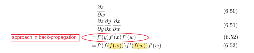 is clearly preferable because of its reduced runtime. However, equation 6.53 is also a valid implementation of the chain rule, and is useful when memory is limited.” (Goodfellow, Bengio)
Implementing Softmax Correctly
- Problem: Exponentials get very big and can have very different magnitudes
- Solution:
- Evaluate $\ln{(\sum_{j=1}^K\exp{(\mathbf{w}_j^\top\mathbf{x})})}$ in the denominator before calculating the fraction
- since $\text{softmax}(\mathbf{a} + \mathbf{b}) = \text{softmax}(\mathbf{a})$ for all $\mathbf{b}\in\mathbb{R}^D$, one can subtract the largest $\mathbf{w}_j$ from the others
- (entspricht $\mathbf{a}=\mathbf{w}_j^\top\mathbf{x}$ und $\mathbf{b}=\mathbf{w}_M^\top\mathbf{x}$ bzw. Kürzen des Bruches mit $\exp{(\mathbf{w}_M^\top\mathbf{x})}$, wobei $\mathbf{w}_M$ das größte weight ist)
- (egal, ob $\mathbf{b}$ von $\mathbf{x}$ abhängt oder nicht!)
- Solution:
MLP in numpy from scratch
- see here
Stochastic Learning vs Batch Learning
source: LeCun et al. “Efficient BackProp”
SGD
- Pros:
- is usually much faster than batch learning
- consider large redundant data set
- example: training set of size 1000 is inadvertently composed of 10 identical copies of a set with 100 samples
- consider large redundant data set
- also often results in better solutions because of the noise in the updates
- because the noise present in the updates can result in the weights jumping into the basin of another, possibly deeper, local minimum. This has been demonstrated in certain simplified cases
- can be used for tracking changes
- useful when the function being modeled is changing over time
- is usually much faster than batch learning
- Cons:
- noise also prevents full convergence to the minimum
- Instead of converging to the exact minimum, the convergence stalls out due to the weight fluctuations
- size of the fluctuations depend on the degree of noise of the stochastic updates:
- The variance of the fluctuations around the local minimum is proportional to the learning rate $\eta$
- So in order to reduce the fluctuations we can either
- decrease (anneal) the learning rate or
- have an adaptive batch size.
- noise also prevents full convergence to the minimum
Batch GD
- Pros:
- Conditions of convergence are well understood.
- Many acceleration techniques (e.g. conjugate gradient) only operate in batch learning. - Theoretical analysis of the weight dynamics and convergence rates are simpler
- one is able to use second order methods to speed the learning process
- Second order methods speed learning by estimating not just the gradient but also the curvature of the cost surface. Given the curvature, one can estimate the approximate location of the actual minimum.
- Cons:
- redundancy can make batch learning much slower than on-line
- often results in worse solutions because of the absence of noise in the updates
- will discover the minimum of whatever basin the weights are initially placed
- changes go undetected and we obtain rather bad results since we are likely to average over several rules
Mini-batch GD
- Another method to remove noise [in SGD] is to use “mini-batches”, that is, start with a small batch size and increase the size as training proceeds.
- However, deciding the rate at which to increase the batch size and which inputs to include in the small batches is as difficult as determining the proper learning rate. Effectively the size of the learning rate in stochastic learning corresponds to the respective size of the mini batch.
- Note also that the problem of removing the noise in the data may be less critical than one thinks because of generalization. Overtraining may occur long before the noise regime is even reached.